| Issue |
A&A
Volume 647, March 2021
|
|
|---|---|---|
| Article Number | A167 | |
| Number of page(s) | 13 | |
| Section | Stellar structure and evolution | |
| DOI | https://doi.org/10.1051/0004-6361/202039596 | |
| Published online | 29 March 2021 | |
Evolved massive stars at low-metallicity
IV. Using the 1.6 μm H-bump to identify red supergiant stars: Case study of NGC 6822⋆
1
IAASARS, National Observatory of Athens, Vas. Pavlou and I. Metaxa, Penteli 15236, Greece
e-mail: This email address is being protected from spambots. You need JavaScript enabled to view it.
2
Department of Astronomy, Beijing Normal University, Beijing 100875, PR China
3
Key Laboratory of Space Astronomy and Technology, National Astronomical Observatories, Chinese Academy of Sciences, Beijing 100101, PR China
4
Rhea Group for ESA/ESAC, Camino Bajo del Castillo, s/n, Urbanizacion Villafranca del Castillo, Villanueva de la Canada, 28692 Madrid, Spain
5
Institute of Astrophysics, Foundation for Research and Technology-Hellas, Heraklion 71110, Greece
6
CAS Key Laboratory of Optical Astronomy, National Astronomical Observatories, Chinese Academy of Sciences, Datun Road 20A, Beijing 100101, PR China
Received:
5
October
2020
Accepted:
20
January
2021
Abstract
We present a case study in which we used a novel method to identify red supergiant (RSG) candidates in NGC 6822 based on their 1.6 μm H-bump. We collected 32 bands of photometric data for NGC 6822 ranging from the optical to the mid-infrared, derived from Gaia, PS1, LGGS, VHS, UKIRT, IRSF, HAWK-I, Spitzer, and WISE. Using the theoretical spectra from MARCS, we demonstrate that there is a prominent difference around 1.6 μm (H-bump) between targets with high and low surface gravity (HSG and LSG). Taking advantage of this feature, we identify efficient color–color diagrams of rzH (r − z vs. z − H) and rzK (r − z vs. z − K) to separate HSG (mostly foreground dwarfs) and LSG targets (mainly background red giant stars, asymptotic giant branch stars, and RSGs) from crossmatching of optical and near-infrared (NIR) data. Moreover, synthetic photometry from ATLAS9 gives similar results. We further separated RSG candidates from the remaining LSG candidates as determined by the H-bump method by using semi-empirical criteria on NIR color–magnitude diagrams, where both the theoretic cuts and morphology of the RSG population are considered. This separation produced 323 RSG candidates. The simulation of foreground stars with Besançon models also indicates that our selection criteria are largely free from the contamination of Galactic giants. In addition to the H-bump method, we used the traditional BVR method (B − V vs. V − R) as a comparison and/or supplement by applying a slightly aggressive cut to select as many RSG candidates as possible (358 targets). Furthermore, the Gaia astrometric solution was used to constrain the sample, where 181 and 193 targets were selected with the H-bump and BVR method, respectively. The percentages of selected targets in the two methods are similar at ∼60%, indicating a comparable accuracy of the two methods. In total, there are 234 RSG candidates after combining targets from the two methods, and 140 (∼60%) of them are in common. The final RSG candidates are in the expected locations on the mid-infrared color–magnitude diagram with [3.6]−[4.5] ≲ 0 and J − [8.0] ≈ 1.0. The spatial distribution is also coincident with the far-ultraviolet-selected star formation regions, suggesting that the selection is reasonable and reliable. We indicate that our method can also be used to identify other LSG targets, such as red giants and asymptotic giant branch stars, and it can also be applied to most of the nearby galaxies by using recent large-scale ground-based surveys. Future ground- and space-based facilities may promote its application beyond the Local Group.
Key words: infrared: stars / galaxies: dwarf / stars: late-type / stars: massive / stars: mass-loss / stars: variables: general
Full Appendix tables are only available at the CDS via anonymous ftp to cdsarc.u-strasbg.fr (130.79.128.5) or via http://cdsarc.u-strasbg.fr/viz-bin/cat/J/A+A/647/A167
© ESO 2021
1. Introduction
Red supergiant stars (RSGs) are helium-fusing evolved massive stars with an initial mass of about 7 ∼ 25 M⊙ (Levesque et al. 2005; Ekström et al. 2013). They represent an extremity of stellar evolution as the coldest and largest members of the massive star population. Their mass-loss rate (MLR) determines their lifetime and whether they end as hydrogen-rich type II-P supernovae (SN) or exit the RSG phase during core He and shell H fusion and evolve backward to the blue end of the Hertzsprung–Russell (H–R) diagram, producing the so-called blue loop (Massey 2013; Smith 2014). Currently, the underlying physics of the blue loop is still largely uncertain. One explanation involves the opposite mirror effect with an expanding He core and a contracting H envelope, but (as with other evolutionary stages) it may also be related to other factors such as treatments of rotation, mixing, overshooting, metallicity, and MLR (Meynet et al. 2015). RSGs are also expected to be in a key stage for the formation of interacting binaries (Neugent et al. 2020). With their high luminosities (≳104 L⊙) and consequently bright magnitudes in the optical and near-infrared (NIR) bands, they can easily be observed beyond our Milky Way (MW; Bergemann et al. 2012). With such an important role in the stellar physics, the investigation of the physical properties and evolution of RSGs has achieved good progress in the past half century (Humphreys & Davidson 1979; Massey & Olsen 2003; González-Fernández et al. 2015; Davies et al. 2017).
To better understand the nature of the RSGs, it is crucial to build a representative sample covering wide ranges of metallicity and luminosity. However, the main challenge of identifying extragalactic RSGs is the foreground contamination from galactic dwarfs and giants. Massey (1998) adopted a simple but effective way to distinguish between foreground dwarfs with high surface gravity (HSG) and background supergiants with low surface gravity (LSG) using a color–color diagram (CCD) of V − R vs. B − V (BVR) in the Johnson filter set. This was mainly based on the line-blanketing effect, which was particularly notable in the B band because a number of weak metal lines lie in the regime. For stars with LSG (e.g., RSGs), weak metal absorption lines decrease the flux in the B band proportionally more than for stars with HSG (e.g., dwarfs), and so it is possible to distinguish LSG and HSG stars by comparing the relative flux in the B band. However, as future observations are gradually moving away from the traditional Johnson filter set (and explore nonoptical wavelength regimes), the modern filter sets have different effective wavelengths and coverages than the Johnson system. In this sense, similar CCDs do not resemble the same effect in the BVR diagram. It is therefore necessary to find new combinations of colors to separate LSGs from HSGs in order to use the data from the most recent large-scale surveys.
We selected NGC 6822 for a case study because it has a rich reservoir of multiwavelength data. As a member of the Local Group (LG), NGC 6822 is an isolated dwarf irregular galaxy (dIrr), which is similar to the Small Magellanic Cloud (SMC) in both size and metallicity (Tolstoy et al. 2001; Cioni & Habing 2005; McConnachie 2012; García-Rojas et al. 2016). With a distance modulus of about 23.40 ± 0.05 (Feast et al. 2012; Rich et al. 2014), it is one of the nearest dwarf galaxies in the LG. Moreover, previous studies (e.g., Levesque & Massey 2012; Patrick et al. 2015) have spectroscopically identified several RSGs in NGC 6822, making it a perfect testbed for our purpose. In this paper, we present our new method based on the H-bump around 1.6 μm, which is a distinct humped spectral feature of LSG targets caused by an apparently lower opacity in the H− of LSGs than HSGs, to identify RSG candidates in NGC 6822. The multiwavelength data and identification of RSG candidates are presented in Sects. 2 and 3, respectively. The candidates are evaluated in Sect. 4. The summary is given in Sect. 5.
2. Multiwavelength data for NGC 6822
We collected multiwavelength data in 32 bands ranging from the optical to the mid-infrared (MIR) for NGC 6822. The MIR data were collected from Khan et al. (2015), who presented Spitzer/Infrared Array Camera (IRAC) [3.6], [4.5], [5.8], [8.0], and Multiband Imaging Photometer (MIPS). Harris & Zaritsky (2009) point-source catalogs for seven galaxies, and the ALLWISE catalog (Cutri et al. 2013) from the Wide-field Infrared Survey Explorer (WISE; Wright et al. 2010). The NIR data were collected from Sibbons et al. (2012) with deep high-quality JHK photometry obtained with the WFCAM on the United Kingdom Infra-Red Telescope (UKIRT), the Visible and Infrared Survey Telescope for Astronomy (VISTA) Hemisphere Survey (VHS) Data Release 6 (DR6; McMahon et al. 2013), Whitelock et al. (2013) with a 3.5 yr survey of the central regions of the NGC 6822 obtained with the Infrared Survey Facility (IRSF) equipped with the SIRIUS camera, and Libralato et al. (2014) with high-precision JKS photometry obtained with the High Acuity Wide-field K-band Imager (HAWK-I) on the ESO Very Large Telescope (VLT). The optical photometric data were collected from two large surveys of the Panoramic Survey Telescope and Rapid Response System (Pan-STARRS, PS1; Chambers et al. 2016) DR2 and Gaia DR2 (Gaia Collaboration 2016, 2018), and the dedicated Local Group Galaxy Survey (LGGS; Massey et al. 2007) for observing nearby galaxies currently forming stars.
As different surveys cover different fields of view (FoVs), we tended to define a common region in which all the surveys overlapped, without excessive sky coverage. Limiting the FoV would allow us to largely reduce the total foreground contamination. Figure 1 shows the common region based on the LGGS that all other surveys either share or in which they are located. Compared to the original dataset of Sibbons et al. (2012), it was only ∼13.5% of the sky area and ∼17.3% of total number of targets, for which the overwhelming majority of foreground stars were excluded.
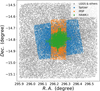 |
Fig. 1. Common observational region of NGC 6822 based on the LGGS. Different colors indicate different surveys. |
In order to reduce the false-positive rate in the following analysis, following the procedure of Yang et al. (2019), each collected dataset was preprocessed and self-deblended with a search radius of 2″ as shown below (from each dataset, targets with neighbors within 2″ were excluded). The deblending radius of 2″ was justified based on the moderate angular resolution of ∼1.8″ of Spitzer. A search radius of 1″ was used for further crossmatching between different datasets as shown below: 28 824 targets from Khan et al. (2015), all of them have 3σ detections in [3.6] and [4.5] bands, but not necessarily in [5.8], [8.0], and Harris & Zaritsky (2009) bands; 7464 targets from the ALLWISE catalog in the common region, with a signal-to-noise ratio (S/N) higher than 3 in the [3.4] and [4.5] bands, but not necessarily in the Dye et al. (2018) and Gustafsson et al. (2008) bands; 25 848 targets from Sibbons et al. (2012) in the common region, with flags of −1 (stellar) or −2 (probably stellar) and photometric errors ≤0.3 mag in the JHK bands; 16 903 targets from VHS DR6 with −3 ≤ mergedClassStat ≤ 3 (merged stellarness-of-profile statistic), mergedClass = −1 (stellar) or −2 (probably stellar), and photometric errors ≤0.3 mag in the JKS bands; 5657 targets from Whitelock et al. (2013) (only deblended, no other constraints); 4318 targets from Libralato et al. (2014), with flags of Jw(Kw) ≠ 0 (weed-out flag with 0 being rejected), q_Jmag(q_Kmag) ≤ 0.25 (quality of the point-spread function (PSF) fit), and photometric errors ≤0.3 mag in the JKS bands; 23 977 targets from PS1 DR2, with flags of nDetections > 2 (number of single-epoch detections in all filters), qualityflag < 64 (flag denoting whether this object is real or a likely false positive), g(r, i, z)QfPerfect > 0.75 (maximum PSF-weighted fraction of pixels that are entirely unmasked from g(r, i, z) filter detections), and rmeanpsfmag − rmeankronmag < 0.05 (a rough cut to separate stars and galaxies); 22 826 targets from Gaia DR2 (only deblended, no other constraints); 43 584 targets from LGGS, with photometric errors ≤0.3 mag in B, V, and R bands.
The catalogs for each dataset are listed in Appendix A. There is a general problem for joining multiple catalogs in that a large number of false-positive matches may appear for targets listed in different surveys. We therefore did not intend to join all catalogs into a common master catalog, but leave the decision to the users. This is a complicated technical issue and a natural outcome of our (or any other) multiwavelength catalogs. We chose not to build a master catalog for three main reasons. The first reason is the lack of reference catalogs in NGC 6822. Unlike Yang et al. (2019, 2021), who built up source catalogs based on Gaia and Spitzer to study bona fide dusty massive stars in the Magellanic Clouds, there is no comprehensive and reliable reference catalog for NGC 6822. For example, Gaia data are insufficient to determine the membership of a considerable part of the targets in NGC 6822, as mentioned in Sect. 4, while Spitzer data are dominated by the background galaxies at the faint magnitude (e.g., [3.6] > 16 mag; Ashby et al. 2009; Williams et al. 2015). Second, different surveys have not necessarily observed the same population of targets because of different wavelengths, sensitivities, depths, sky coverages, quality cuts, and so on. For example, dusty targets may be extremely faint and undetected at short wavelengths (e.g., B or even V band), but are very bright at long wavelengths (e.g., IR bands). Even for similar wavelengths, some targets may be available in one survey but not necessarily in others, for example, because of different exposure times and quality cuts. Third, we could build up a master catalog (we did try) by simply joining all catalogs by using their coordinates, for which each match represents a group of friends of friends. However, it is important to note that for any particular pair in a matched group, there is no guarantee that the two objects match, but only that it can hop from one to the other through pairs that do match1. This shows that a master catalog creates false matches, especially at faint magnitudes and crowded regions. Our goal is to study RSGs, therefore false positives are generally not a great problem because RSGs are bright and we have deblended each dataset.
3. Identifying red supergiant stars using the H-bump at 1.6 μm
To identify RSGs in NGC 6822, we first used the theoretical spectra from MARCS, which is an one-dimensional, hydrostatic, spherical, local thermodynamic equilibrium model atmospheres (Plez 2003; Gustafsson et al. 2003, 2008), to demonstrate the general separation between HSG (e.g., dwarfs) and LSG (e.g., supergiants) targets. MARCS models were widely used in recent studies to fit moderate-resolution spectrophotometry of RSGs in the MW, the MCs, M 31, and so on (Levesque et al. 2005, 2006; Massey et al. 2009; Davies et al. 2013). Figure 2 shows two normalized resampled spectra with the same effective temperature (Teff) of 3700 K at a metallicity (Z) of −0.75 but for different surface gravities (Log g) of 4.5 (HSG) and 0.0 (LSG). The diagram shows an obvious difference (∼25% of normalized flux) between the HSG and LSG targets caused by the humped spectral feature of LSG targets around 1.6 μm (H-bump). This H-bump is expected to appear in cool stars because the opacity in the H− of supergiants (or giants) is apparently lower than dwarfs (although they are both at a minimum of the H− opacity). However, this is suppressed at high metallicities by molecular absorption (e.g., CO; John 1988; Davies et al. 2013). Thus, in principle, a color combination involving at least one of the JHKS filters (as shown in the diagram) can be used to distinguish between foreground dwarfs and background supergiants. The dwarfs in NGC 6822 do not affect the result because they are much fainter than foreground dwarfs and supergiants in the same galaxy.
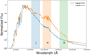 |
Fig. 2. Two normalized resampled MARCS spectra with the same Teff = 3700 K at a metallicity of −0.75, but for different surface gravities of 4.5 (HSG) and 0.0 (LSG). The LSG target shows a humped spectral feature around 1.6 μm (H-bump). The approximate wavelength ranges of JHKS filters are shown as different shades. |
To test this assumption, we crossmatched data from PS1 and Sibbons et al. (2012) (UKIRT) with a search radius of 1″, which resulted in 15 508 targets. The MARCS spectra (Teff = 3300, 3400, 3500, 3600, 3700, 3800, 3900, 4000, 4250 K; Log g = 0.0, 4.5; Z = −0.75, 0.0) were resampled and convolved with filters from the PS1 and UKIRT. The magnitudes and colors were all in the WFCAM instrumental system (Hodgkin et al. 2009). We investigated all color combinations from PS1 and UKIRT, finding that two of them (z − H vs. r − z (rzH) and z − K vs. r − z (rzK)) successfully separated foreground HSG dwarfs from background LSG targets, as shown in Fig. 3 (we note that in contrast, the color combinations involved in the J filter were not as good as in H and K). The diagram shows that the expected color–color distributions of LSG targets (Log g ∼ 0.0) are coincident with the observational data after applying appropriate extinction (we adopted AV = 1.0 mag as a combination of foreground and intrinsic extinction with E(r − z) = 0.356, E(z − h) = 0.356, and E(z − K) = 0.409 for NGC 6822; Wang & Chen 2019). Initially, we used several statistics methods (e.g., kernel density estimation (KDE), median absolute deviation (MAD), histogram, and so on) to quantitatively separate the HSG and LSG regions. However, all of the methods failed to include all the spectroscopically confirmed RSGs from Levesque & Massey (2012) and Patrick et al. (2015). The upper left panel of Fig. 3 shows examples of KDE and MAD. For KDE, LSG are separated well from HSG targets, but a few spectroscopically confirmed RSGs are not included that are located directly in the middle of the HSG and LSG populations. For MAD, it properly represents the HSG population for the most part, but fails at the junction of the HSG and LSG populations. We therefore finally defined the LSG region by eye as
 (1)
(1)
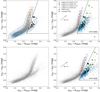 |
Fig. 3. Color–color diagrams of z − H vs. r − z (upper) and z − K vs. r − z (bottom). Upper left panel: examples of KDE (contours) and MAD (solid circles indicate the median values of z − H color in equal bins (from 0.3 to 2.6 with a step of 0.2 mag) of the r − z color, and the error bars indicate three times of MAD for the corresponding bin), both of which fail to include all the spectroscopically confirmed RSGs. Left panels: original data without the overlapping MARCS models, right panels: MARCS-model selected LSG region (dashed lines are hand-drawn). Small and large solid circles and diamonds represent HSG and LSG targets at different Teff (from 3300 to 4250 K) in different metallicities derived from MARCS models, respectively. Spectroscopically confirmed RSGs from Levesque & Massey (2012) and Patrick et al. (2015) are shown as open pentagon and solid stars, respectively. A reddening vector of AV = 1.0 mag is shown as a reference (same below). The error bars in the bottom right corner of the right panels indicate the median error of each color. |
or
 (2)
(2)
and for both CCDs,
 (3)
(3)
We also show the datasets with and without the overlapping models, which clearly indicates that our boundaries were appropriate. Spectroscopically confirmed RSGs from Levesque & Massey (2012) and Patrick et al. (2015) are all located within the LSG region. Moreover, further investigation using synthetic photometry from ATLAS9 models2 (Teff = 3500, 3750, 4000, 4250 K; Log g = 0.0, 4.5; Z = −0.5, 0.0; Castelli & Kurucz 2003) also gave similar results as shown in Fig. 4. In total, we selected 1276 and 1194 LSG targets from rzH and rzK CCDs with 1051 targets in common, respectively.
After collecting LSG targets, we separated RSG candidates from the remaining LSG candidates as determined by the H-bump method because the majority of the LSG targets would be red giants (RGs) or asymptotic giant branch stars (AGBs). This was relatively easy as the selected targets were assumed to be located in the NGC 6822 at the same distance, so that the RSGs would be brighter than RGs and AGBs. The left panel of Fig. 5 shows the CMD of KS vs. J − KS. Previously, we identified the RSG population in the SMC using the theoretical distribution in an NIR CMD, where K1, K2, and KR lines were used to separate the oxygen-rich AGB, carbon-rich AGB, and RSG populations (see more details in Cioni et al. 2006; Boyer et al. 2012; Yang & Jiang 2012, 2011; Yang et al. 2018, 2019, 2020). Here we applied a slightly modified selection criterion based on previous studies. As indicated by Yang et al. (2020), there is a continuum with similarity that overlaps in RSGs and AGBs in spectra, light curves, and CMDs. Thus, the clear separation between them is still a pending issue and cannot be accurately parameterized. The intercept of the K1′ line, which separated RSGs from AGBs, was changed depending on the morphology of the CMD and distance modulus. The nearly vertical branch on the CMD was most likely the RSG population, while the AGB population stretched toward the red end. The  line indicated the blue boundary (Δ(J − K) = 0.333 mag from K1′) of the RSG population. In order to avoid contamination from RGs and AGBs, the lower limit of the magnitude of RSG population (horizontal dotted line) was set to MK = −6.5 mag (K = 16.9 mag; ∼0.5 mag above the K-band tip of RGB (K-TRGB = 17.36 ± 0.04 mag); Hirschauer et al. 2020). However, inevitably, we might lose some low-luminosity RSGs located between our lower limit and the K-TRGB. In addition to the Galactic dwarfs, another source of contamination are RGs in the Galactic halo. To address this issue, we used Besançon models of the MW (Robin et al. 2003) to predict the location of foreground stars along the line of sight of NGC 6822, as shown in the right panel of Fig. 5. The two panels show that our selection largely avoids the majority of Galactic giants contamination, except at the faint end close to the K-TRGB, as expected. In total, we selected 227 RSG candidates based on the combination of CCDs and CMDs from PS1 and UKIRT, where 221 are based on rzH, 200 are based on rzK, and 194 (∼85%) are in common.
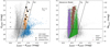 |
Fig. 5. Color–magnitude diagrams of K vs. J − K for observational data (left) and the Besançon models along the line of sight of NGC 6822 (right). Left panel: 227 RSG candidates are selected based on slightly modified selection criteria indicated by the K1′ and |

As different NIR surveys cover different parts of NGC 6822 with different sensitivities, depths, and quality cuts, they may complement each other. We therefore also crossmatched PS1 with other NIR data. The crossmatch of PS1 and VHS/IRSF/HAWK-I resulted in 11 515, 2207, and 958 targets. We selected 211 RSG candidates based on PS1 vs. VHS (Fig. B.1; no H-band data from VHS), 183 RSG candidates based on PS1 vs. IRSF (Fig. B.2; 176 based on rzH, 178 based on rzKS, and 171 in common), and 88 RSG candidates based on PS1 vs. HAWK-I (Fig. B.3; no H-band data from HAWK-I). We present all the CCDs and CMDs in Appendix B. Despite the slight differences in the filter sets (e.g., HKS between UKIRT, VISTA, IRSF, and HAWK-I), they all give similar results. This means that any HKS filters can be used in future studies. We only compared NIR filters because the differences are much smaller between optical filters than the NIR filters. After duplicates were removed, 323 RSG candidates are based on PS1 and NIR data.
In addition to the H-bump method that we adopted to identify RSG candidates, we also applied the traditional BVR method as a comparison and/or supplement. Figure 6 shows the BVR CCD and R vs. V − R CMD. Here we used slightly aggressive cuts (a cut of V ≤ 21.5 mag was applied in order to reduce the contamination) in the CCD to select as many RSG candidates as possible because the sample would be further constrained by the CMD. The cuts in the CMD were made by eye in order to select the RSG branch based on its morphology, which is due to the ambiguous boundary between RSGs and AGBs, as mentioned before. The lower limit of the magnitude of the RSG population was set to MR = −3.5 mag (R = 19.9 mag; about half a magnitude above the R-TRGB ≈ 20.6 mag, which was roughly determined by the saddle-point method; Ren et al. 2021). Similar simulations from the Besançon models have indicated that the selection of RSG candidates was also largely free from foreground contamination of giants. In total, we selected 358 RSG candidates based on LGGS data.
4. Constraining the red supergiant candidates
We further constrained the RSG candidates using the Gaia astrometric solution. The RSG candidates from both methods were crossmatched with Gaia DR2 with a search radius of 1″, which resulted in 309 targets for the H-bump and 314 targets for the BVR method. Targets without Gaia data were not considered for further analysis. For the members of NGC 6822, the proper motions (PMs) and parallaxes of targets were assumed to be around zero. We therefore constrained the Gaia astrometric solution and color of the final RSG candidates as listed in Table 1. The constraints are justified based on the typical errors of ∼1.2 mas yr−1 for the PMs and ∼0.7 mas for the parallaxes at the faint end of the Gaia magnitude (Lindegren et al. 2018). We did not apply the same statistical method in Yang et al. (2019), where we used Gaussian profiles to fit the Gaia astrometric solution in order to select the proper members of the SMC.
Constraints of the Gaia astrometric solution and color for the final RSG sample.
This is mainly due to two reasons. First, for the SMC (or any other nearby galaxy with large angular size and relatively high Galactic latitude), the dominant population in the FoV consists of the members of the target galaxy. However, for the case of NGC 6822 with its relatively small angular size and low Galactic latitude (it is also more distant than the SMC), the dominant population no longer consists of its members but of foreground stars. Second, a large fraction of the members of NGC 6822 do not have proper astrometric measurements either due to faintness or crowding (it is estimated that the members of NGC 6822 only comprise around 10% of the population of the measurable astrometric solution in the FoV based on Fig. 7). The statistics of the astrometric solution in the FoV will therefore be highly biased by the high contamination of foreground stars.
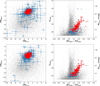 |
Fig. 7. Evaluation of the Gaia astrometric solution (left) and CMDs (right) for RSG candidates from H-bump (top) and BVR method (bottom). The final selected RSG candidates (red) are clustered around zero in PMs, while outliers (blue) are mainly at the faint and blue end of the CMDs. |
Figure 7 shows the constraints on the Gaia astrometric solution and CMDs for the H-bump and BVR method. We selected 181 and 193 targets with the H-bump and BVR method, respectively. The selected targets are concentrated around PMs of zero, and are mainly limited to GGaia ≈ 20.0 mag due to the relatively strict constraints of the Gaia astrometric solution, as mentioned above. The outliers, as expected, are mostly located at the faint end on the CMDs because of large PMs (parallax) and/or large PM (parallax) errors. We note that among the blue outlier points, some genuine RSGs are expected to exist. It might be argued that faint targets without Gaia astrometric solution might also belong to NGC 6822 because of their distances. However, another possibility is that they are the distant Galactic red dwarfs, especially because NGC 6822 lies at a relatively low Galactic latitude. The foreground contamination can be mitigated by taking conservative cuts in the CCD, CMD, and astrometric solution. However, it will also cause target loss at the faint and blue end. The percentages of selected targets in both methods are similar: ∼59% (181/309) for the H-bump and ∼61% (193/314) for the BVR method, which indicates that the accuracy of the two methods is comparable. In total, there are 234 RSG candidates when the targets from both methods are combined, and 140 (∼60%) of them are in common. The full information for the 234 candidates is listed in Table 2. We note that there is a large difference for the number of RSG candidates between NGC 6822 and the SMC (1239 candidates; Yang et al. 2020), even though they are similar in sizes and metallicities. The large number of RSG candidates in the SMC is most likely due to the interaction between the MW, the LMC, and the SMC, which triggered multiple peaks of star formation in the past few hundred million years (an underlying constant SFR of ∼0.1 M⊙ yr−1 with superposed episodes of enhanced star formation at 2−3 Gyr, 400 Myr, and 60 Myr; Yoshizawa & Noguchi 2003; Harris & Zaritsky 2004, 2009; Indu & Subramaniam 2011). Because NGC 6822 is an isolated dIrr, its star formation rate is relatively low and constant (∼0.014 M⊙ yr−1 over the past 100 Myr, and ∼0.01 M⊙ yr−1 in the most recent 10 Myr Wyder 2001; Efremova et al. 2011; Fusco et al. 2014), resulting in a small number of RSG candidates.
Final sample of 234 RSG candidates in NGC 6822.
In addition to previous optical and NIR CMDs, we also plot MIR CMDs dominated by the dust emission to further evaluate the sample. Figure 8 show CMDs of [4.5] vs. [3.6]−[4.5], [8.0] vs. J − [8.0], and Harris & Zaritsky (2009) vs. K − [24]. Background targets are the result of crossmatching (1″ search radius) between Spitzer and UKIRT data, without upper limit and extended targets (|[3.6]PSF − [3.6]Aper|≤0.1). The selected RSG candidates are all in the expected locations (see Fig. 5 of Yang et al. 2020), with blue (≲0) in [3.6]−[4.5] and red (∼1.0) in J − [8.0]. The spread in K − [24] is most likely due to the low sensitivity in the Harris & Zaritsky (2009) band. Finally, Fig. 9 shows the spatial distribution of RSG candidates, which follows the far-ultraviolet (FUV) selected star formation regions from Efremova et al. (2011) well. This also indicates that our selection of RSG candidates is reasonable and reliable. The comparison of the spatial distribution of our sample and the result from Hirschauer et al. (2020; see Fig. 12 of their paper) may indicate that our sample is purer with less contamination from low-mass and foreground stars because the distribution of RSGs from Hirschauer et al. (2020) is less compact.
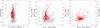 |
Fig. 8. Mid-infrared CMDs of [4.5] vs. [3.6]−[4.5] (left), [8.0] vs. J − [8.0] (middle), and Harris & Zaritsky (2009) vs. K − [24] (right). The RSG candidates are located in the expected position in each diagram at [3.6]−[4.5] ≲ 0 and J − [8.0] ≈ 1.0. The large spread in K − [24] is most likely due to the low sensitivity in the Harris & Zaritsky (2009) band. |
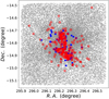 |
Fig. 9. Spatial distribution of RSG candidates (open red circles). It follows nicely the distribution of FUV-selected star formation regions (solid blue squares; Efremova et al. 2011). |
Finally, we would like to point out that our method can also be used to identify other LSG targets such as RGs and AGBs, as shown in Fig. 5. Combining the high-resolution and deep photometry from most recent large-scale ground-based surveys, for example, VHS, UKIRT Hemisphere Survey (UHS; Dye et al. 2018), UKIRT Infrared Deep Sky Survey (UKIDSS; Lawrence et al. 2007), PS1, Legacy Survey (Dey et al. 2019), using the H-bump to identify RSGs with non-Johnson filter bands can be largely applied to most of the nearby galaxies. A good example of our method has been shown in Ren et al. (2021). Moreover, future ground- and space-based facilities, such as the Chinese Space Station Telescope (CSST), the Vera C. Rubin Observatory (LSST), Euclid, the Nancy Grace Roman Space Telescope (NGRST), and the James Webb Space Telescope (JWST), may promote further application beyond the LG, uncovering unprecedented populations of RSGs in a vast range of different galactic environments.
5. Summary
We presented a novel method for identifying RSG candidates based on their 1.6 μm H-bump, for which a case study was carried out for NGC 6822 because of its rich reservoir in multiwavelength data. Thirty-two bands of data were collected, ranging from optical to MIR, derived from Gaia, PS1, LGGS, VHS, UKIRT, IRSF, HAWK-I, Spitzer, and WISE.
The theoretical spectra of LSG and HSG targets from MARCS were compared, which indicated a striking difference (around the 1.6 μm H-bump) in the two populations. To take advantage of this difference, we crossmatched optical (PS1) and NIR surveys to identify efficient color combinations that separate LSG (mostly foreground dwarfs) and HSG targets (mainly background RGs, AGBs, and RSGs). The best results are provided by rzH and rzK. Moreover, synthetic photometry derived from ATLAS9 models also gave similar results. We further separated RSG candidates from the rest using semi-empirical criteria on NIR CMDs, where both the theoretic cuts and morphology of RSG population were considered. Simulations of foreground stars along the line of sight of NGC 6822 with Besançon models also indicated that our selection criteria were largely free from the contamination of Galactic giants. In total, there are 323 RSG candidates based on PS1 and NIR (UKIRT, VHS, IRSF, HAWK-I) data. To test our approach, we also used the traditional BVR method. We applied a slightly aggressive cut in order to select as many RSG candidates as possible, which resulted in 358 targets.
After selecting RSG candidates based on CCDs and CMDs, the Gaia astrometric solution was used to further constrain the sample. We applied relatively strict criteria to Gaia PMs and parallaxes, where 181 and 193 targets were selected for the H-bump and BVR method, respectively. The accuracy of the two methods is comparable at ∼60%. In total, there are 234 RSG candidates when targets from both methods are combined, and 140 (∼60%) of them are in common.
We further evaluated the RSG sample by comparing its location in different MIR CMDs and the spatial distribution. The RSG candidates are found in the expected locations in the MIR CMDs with [3.6]−[4.5] ≲ 0 and J − [8.0] ≈ 1.0. Its spatial distribution coincides with the FUV-selected star formation regions, strengthening our belief that this selection approach is reasonable and reliable.
Finally, we indicate that our method can also be used to identify other LSG targets such as RGs and AGBs, and it can be applied to most of the nearby galaxies using recent large-scale ground-based surveys. Future ground- and space-based facilities may promote its application beyond the LG, uncovering unprecedented populations of RSGs in a vast range of different galactic environments.
Acknowledgments
We would like to thank the anonymous referee for many constructive comments and suggestions. This study has received funding from the European Research Council (ERC) under the European Union’s Horizon 2020 research and innovation programme (grant agreement number 772086). B.W.J and J.G. gratefully acknowledge support from the National Natural Science Foundation of China (Grant No. 11533002 and U1631104). This work is based in part on observations made with the Spitzer Space Telescope, which is operated by the Jet Propulsion Laboratory, California Institute of Technology under a contract with NASA. This publication makes use of data products from the Wide-field Infrared Survey Explorer, which is a joint project of the University of California, Los Angeles, and the Jet Propulsion Laboratory/California Institute of Technology. It is funded by the National Aeronautics and Space Administration. This research has made use of the NASA/IPAC Infrared Science Archive, which is operated by the Jet Propulsion Laboratory, California Institute of Technology, under contract with the National Aeronautics and Space Administration. This work has made use of data from the European Space Agency (ESA) mission Gaia (https://www.cosmos.esa.int/gaia), processed by the Gaia Data Processing and Analysis Consortium (DPAC, https://www.cosmos.esa.int/web/gaia/dpac/consortium). Funding for the DPAC has been provided by national institutions, in particular the institutions participating in the Gaia Multilateral Agreement. This research has made use of the SIMBAD database and VizieR catalog access tool, operated at CDS, Strasbourg, France, and the Tool for OPerations on Catalogues And Tables (TOPCAT; Taylor 2005). This research has made use of the Spanish Virtual Observatory (http://svo.cab.inta-csic.es) supported from the Spanish MICINN/FEDER through grant AyA2017-84089.
References
- Ashby, M. L. N., Stern, D., Brodwin, M., et al. 2009, ApJ, 701, 428 [NASA ADS] [CrossRef] [Google Scholar]
- Bergemann, M., Kudritzki, R.-P., Plez, B., et al. 2012, ApJ, 751, 156 [NASA ADS] [CrossRef] [Google Scholar]
- Boyer, M. L., Srinivasan, S., Riebel, D., et al. 2012, ApJ, 748, 40 [NASA ADS] [CrossRef] [Google Scholar]
- Castelli, F., & Kurucz, R. L. 2003, Model. Stellar Atmos., 210, A20 [Google Scholar]
- Chambers, K. C., Magnier, E. A., Metcalfe, N., et al. 2016, ArXiv e-prints [arXiv:1612.05560] [Google Scholar]
- Cioni, M.-R. L., & Habing, H. J. 2005, A&A, 429, 837 [NASA ADS] [CrossRef] [EDP Sciences] [Google Scholar]
- Cioni, M.-R. L., Girardi, L., Marigo, P., & Habing, H. J. 2006, A&A, 448, 77 [NASA ADS] [CrossRef] [EDP Sciences] [Google Scholar]
- Cutri, R. M., Wright, E. L., Conrow, T., et al. 2013, VizieR Online Data Catalog: II/328 [Google Scholar]
- Davies, B., Kudritzki, R.-P., Plez, B., et al. 2013, ApJ, 767, 3 [NASA ADS] [CrossRef] [Google Scholar]
- Davies, B., Kudritzki, R.-P., Lardo, C., et al. 2017, ApJ, 847, 112 [Google Scholar]
- Dey, A., Schlegel, D. J., Lang, D., et al. 2019, AJ, 157, 168 [NASA ADS] [CrossRef] [Google Scholar]
- Dye, S., Lawrence, A., Read, M. A., et al. 2018, MNRAS, 473, 5113 [NASA ADS] [CrossRef] [Google Scholar]
- Efremova, B. V., Bianchi, L., Thilker, D. A., et al. 2011, ApJ, 730, 88 [NASA ADS] [CrossRef] [Google Scholar]
- Ekström, S., Georgy, C., Meynet, G., Groh, J., & Granada, A. 2013, EAS Publ. Ser., 60, 31 [Google Scholar]
- Feast, M. W., Whitelock, P. A., Menzies, J. W., et al. 2012, MNRAS, 421, 2998 [NASA ADS] [CrossRef] [Google Scholar]
- Fusco, F., Buonanno, R., Hidalgo, S. L., et al. 2014, A&A, 572, A26 [EDP Sciences] [Google Scholar]
- Gaia Collaboration (Prusti, T., et al.) 2016, A&A, 595, A1 [NASA ADS] [CrossRef] [EDP Sciences] [Google Scholar]
- Gaia Collaboration (Brown, A. G. A., et al.) 2018, A&A, 616, A1 [NASA ADS] [CrossRef] [EDP Sciences] [Google Scholar]
- García-Rojas, J., Peña, M., Flores-Durán, S., et al. 2016, A&A, 586, A59 [NASA ADS] [CrossRef] [EDP Sciences] [Google Scholar]
- González-Fernández, C., Dorda, R., Negueruela, I., & Marco, A. 2015, A&A, 578, A3 [NASA ADS] [CrossRef] [EDP Sciences] [Google Scholar]
- Gustafsson, B., Edvardsson, B., Eriksson, K., et al. 2003, Stellar Atmos. Model., 288, 331 [Google Scholar]
- Gustafsson, B., Edvardsson, B., Eriksson, K., et al. 2008, A&A, 486, 951 [NASA ADS] [CrossRef] [EDP Sciences] [Google Scholar]
- Harris, J., & Zaritsky, D. 2004, AJ, 127, 1531 [Google Scholar]
- Harris, J., & Zaritsky, D. 2009, AJ, 138, 1243 [NASA ADS] [CrossRef] [Google Scholar]
- Hirschauer, A. S., Gray, L., Meixner, M., et al. 2020, ApJ, 892, 91 [Google Scholar]
- Hodgkin, S. T., Irwin, M. J., Hewett, P. C., et al. 2009, MNRAS, 394, 675 [NASA ADS] [CrossRef] [Google Scholar]
- Humphreys, R. M., & Davidson, K. 1979, ApJ, 232, 409 [NASA ADS] [CrossRef] [Google Scholar]
- Indu, G., & Subramaniam, A. 2011, A&A, 535, A115 [NASA ADS] [CrossRef] [EDP Sciences] [Google Scholar]
- John, T. L. 1988, A&A, 193, 189 [NASA ADS] [Google Scholar]
- Khan, R., Stanek, K. Z., Kochanek, C. S., et al. 2015, ApJS, 219, 42 [NASA ADS] [CrossRef] [Google Scholar]
- Lawrence, A., Warren, S. J., Almaini, O., et al. 2007, MNRAS, 379, 1599 [NASA ADS] [CrossRef] [MathSciNet] [Google Scholar]
- Levesque, E. M., & Massey, P. 2012, AJ, 144, 2 [CrossRef] [Google Scholar]
- Levesque, E. M., Massey, P., Olsen, K. A. G., et al. 2005, ApJ, 628, 973 [NASA ADS] [CrossRef] [Google Scholar]
- Levesque, E. M., Massey, P., Olsen, K. A. G., et al. 2006, ApJ, 645, 1102 [NASA ADS] [CrossRef] [Google Scholar]
- Libralato, M., Bellini, A., Bedin, L. R., et al. 2014, A&A, 563, A80 [NASA ADS] [CrossRef] [EDP Sciences] [Google Scholar]
- Lindegren, L., Hernández, J., Bombrun, A., et al. 2018, A&A, 616, A2 [NASA ADS] [CrossRef] [EDP Sciences] [Google Scholar]
- Massey, P. 1998, ApJ, 501, 153 [NASA ADS] [CrossRef] [Google Scholar]
- Massey, P. 2013, New Astron. Rev., 57, 14 [NASA ADS] [CrossRef] [Google Scholar]
- Massey, P., & Olsen, K. A. G. 2003, AJ, 126, 2867 [NASA ADS] [CrossRef] [Google Scholar]
- Massey, P., Olsen, K. A. G., Hodge, P. W., et al. 2007, AJ, 133, 2393 [NASA ADS] [CrossRef] [MathSciNet] [Google Scholar]
- Massey, P., Silva, D. R., Levesque, E. M., et al. 2009, ApJ, 703, 420 [NASA ADS] [CrossRef] [Google Scholar]
- McConnachie, A. W. 2012, AJ, 144, 4 [Google Scholar]
- McMahon, R. G., Banerji, M., Gonzalez, E., et al. 2013, The Messenger, 154, 35 [NASA ADS] [Google Scholar]
- Meynet, G., Chomienne, V., Ekström, S., et al. 2015, A&A, 575, A60 [NASA ADS] [CrossRef] [EDP Sciences] [Google Scholar]
- Neugent, K. F., Levesque, E. M., Massey, P., et al. 2020, ApJ, 900, 118 [CrossRef] [Google Scholar]
- Patrick, L. R., Evans, C. J., Davies, B., et al. 2015, ApJ, 803, 14 [NASA ADS] [CrossRef] [Google Scholar]
- Plez, B. 2003, ASP Conf. Ser., 298, 189 [Google Scholar]
- Ren, Y., Jiang, B., Yang, M., et al. 2021, ApJ, 907, 18 [Google Scholar]
- Rich, J. A., Persson, S. E., Freedman, W. L., et al. 2014, ApJ, 794, 107 [NASA ADS] [CrossRef] [Google Scholar]
- Robin, A. C., Reylé, C., Derrière, S., et al. 2003, A&A, 409, 523 [NASA ADS] [CrossRef] [EDP Sciences] [Google Scholar]
- Sibbons, L. F., Ryan, S. G., Cioni, M.-R. L., et al. 2012, A&A, 540, A135 [NASA ADS] [CrossRef] [EDP Sciences] [Google Scholar]
- Smith, N. 2014, ARA&A, 52, 487 [Google Scholar]
- Taylor, M. B. 2005, ASP Conf. Ser., 347, 29 [Google Scholar]
- Tolstoy, E., Irwin, M. J., Cole, A. A., et al. 2001, MNRAS, 327, 918 [Google Scholar]
- Wang, S., & Chen, X. 2019, ApJ, 877, 116 [NASA ADS] [CrossRef] [Google Scholar]
- Whitelock, P. A., Menzies, J. W., Feast, M. W., et al. 2013, MNRAS, 428, 2216 [NASA ADS] [CrossRef] [Google Scholar]
- Williams, S. J., Bonanos, A. Z., Whitmore, B. C., et al. 2015, A&A, 578, A100 [NASA ADS] [CrossRef] [EDP Sciences] [Google Scholar]
- Wright, E. L., Eisenhardt, P. R. M., Mainzer, A. K., et al. 2010, AJ, 140, 1868 [Google Scholar]
- Wyder, T. K. 2001, AJ, 122, 2490 [NASA ADS] [CrossRef] [Google Scholar]
- Yang, M., & Jiang, B. W. 2011, ApJ, 727, 53 [NASA ADS] [CrossRef] [Google Scholar]
- Yang, M., & Jiang, B. W. 2012, ApJ, 754, 35 [NASA ADS] [CrossRef] [Google Scholar]
- Yang, M., Bonanos, A. Z., Jiang, B.-W., et al. 2018, A&A, 616, A175 [NASA ADS] [CrossRef] [EDP Sciences] [Google Scholar]
- Yang, M., Bonanos, A. Z., Jiang, B.-W., et al. 2019, A&A, 629, A91 [CrossRef] [EDP Sciences] [Google Scholar]
- Yang, M., Bonanos, A. Z., Jiang, B.-W., et al. 2020, A&A, 639, A116 [NASA ADS] [CrossRef] [EDP Sciences] [Google Scholar]
- Yang, M., Bonanos, A. Z., Jiang, B., et al. 2021, A&A, 646, A141 [EDP Sciences] [Google Scholar]
- Yoshizawa, A. M., & Noguchi, M. 2003, MNRAS, 339, 1135 [NASA ADS] [CrossRef] [Google Scholar]
Appendix A: Photometric catalogs of nine datasets
We list here the examples of nine photometric catalogs from Sect. 2. All tables are available in their entireties at the CDS.
PS1 photometric catalog.
Gaia photometric catalog.
LGGS photometric catalog.
UKIRT photometric catalog.
VHS photometric catalog.
IRSF photometric catalog.
HAWK-I photometric catalog.
Spitzer photometric catalog.
WISE photometric catalog.
Appendix B: Additional color–color and color–magnitude diagrams
We present here additional CCDs and CMDs from PS1 vs. VHS, PS1 vs. IRSF, and PS1 vs. HAWK-I. Each dataset is reduced following the same procedure as described in Sect. 3.
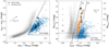 |
Fig. B.1. Same as Figs. 3 and 5, but for the combination of PS1 and VHS data. 211 RSG candidates are selected. |
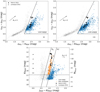 |
Fig. B.2. Same as Figs. 3 and 5, but for the combination of PS1 and IRSF data. 183 RSG candidates are selected, 176 based on rzH, 178 based on rzKS, and 171 in common. |
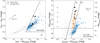 |
Fig. B.3. Same as Figs. 3 and 5, but for the combination of PS1 and HWAK-I data. 88 RSG candidates are selected. |
All Tables
Constraints of the Gaia astrometric solution and color for the final RSG sample.
All Figures
|
Fig. 1. Common observational region of NGC 6822 based on the LGGS. Different colors indicate different surveys. |
| In the text | |
|
Fig. 2. Two normalized resampled MARCS spectra with the same Teff = 3700 K at a metallicity of −0.75, but for different surface gravities of 4.5 (HSG) and 0.0 (LSG). The LSG target shows a humped spectral feature around 1.6 μm (H-bump). The approximate wavelength ranges of JHKS filters are shown as different shades. |
| In the text | |
|
Fig. 3. Color–color diagrams of z − H vs. r − z (upper) and z − K vs. r − z (bottom). Upper left panel: examples of KDE (contours) and MAD (solid circles indicate the median values of z − H color in equal bins (from 0.3 to 2.6 with a step of 0.2 mag) of the r − z color, and the error bars indicate three times of MAD for the corresponding bin), both of which fail to include all the spectroscopically confirmed RSGs. Left panels: original data without the overlapping MARCS models, right panels: MARCS-model selected LSG region (dashed lines are hand-drawn). Small and large solid circles and diamonds represent HSG and LSG targets at different Teff (from 3300 to 4250 K) in different metallicities derived from MARCS models, respectively. Spectroscopically confirmed RSGs from Levesque & Massey (2012) and Patrick et al. (2015) are shown as open pentagon and solid stars, respectively. A reddening vector of AV = 1.0 mag is shown as a reference (same below). The error bars in the bottom right corner of the right panels indicate the median error of each color. |
| In the text | |
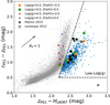 |
Fig. 4. Same as Fig. 3, but for models from ATLAS9 at Teff = 3500, 3750, 4000, 4250 K. |
| In the text | |
|
Fig. 5. Color–magnitude diagrams of K vs. J − K for observational data (left) and the Besançon models along the line of sight of NGC 6822 (right). Left panel: 227 RSG candidates are selected based on slightly modified selection criteria indicated by the K1′ and |
| In the text | |
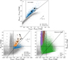 |
Fig. 6. Same as Figs. 3 and 5, but for LGGS data. 358 RSG candidates are selected. |
| In the text | |
|
Fig. 7. Evaluation of the Gaia astrometric solution (left) and CMDs (right) for RSG candidates from H-bump (top) and BVR method (bottom). The final selected RSG candidates (red) are clustered around zero in PMs, while outliers (blue) are mainly at the faint and blue end of the CMDs. |
| In the text | |
|
Fig. 8. Mid-infrared CMDs of [4.5] vs. [3.6]−[4.5] (left), [8.0] vs. J − [8.0] (middle), and Harris & Zaritsky (2009) vs. K − [24] (right). The RSG candidates are located in the expected position in each diagram at [3.6]−[4.5] ≲ 0 and J − [8.0] ≈ 1.0. The large spread in K − [24] is most likely due to the low sensitivity in the Harris & Zaritsky (2009) band. |
| In the text | |
|
Fig. 9. Spatial distribution of RSG candidates (open red circles). It follows nicely the distribution of FUV-selected star formation regions (solid blue squares; Efremova et al. 2011). |
| In the text | |
|
Fig. B.1. Same as Figs. 3 and 5, but for the combination of PS1 and VHS data. 211 RSG candidates are selected. |
| In the text | |
|
Fig. B.2. Same as Figs. 3 and 5, but for the combination of PS1 and IRSF data. 183 RSG candidates are selected, 176 based on rzH, 178 based on rzKS, and 171 in common. |
| In the text | |
|
Fig. B.3. Same as Figs. 3 and 5, but for the combination of PS1 and HWAK-I data. 88 RSG candidates are selected. |
| In the text | |
Current usage metrics show cumulative count of Article Views (full-text article views including HTML views, PDF and ePub downloads, according to the available data) and Abstracts Views on Vision4Press platform.
Data correspond to usage on the plateform after 2015. The current usage metrics is available 48-96 hours after online publication and is updated daily on week days.
Initial download of the metrics may take a while.