| Issue |
A&A
Volume 646, February 2021
|
|
|---|---|---|
| Article Number | A111 | |
| Number of page(s) | 14 | |
| Section | Extragalactic astronomy | |
| DOI | https://doi.org/10.1051/0004-6361/202039396 | |
| Published online | 16 February 2021 | |
Speed limits for radiation-driven SMBH winds
1
Department of Physics, University of Rome “Tor Vergata”, Via della Ricerca Scientifica 1, 00133 Rome, Italy
2
INAF – Osservatorio Astronomico di Roma, Via Frascati 33, 00078 Monte Porzio Catone, Italy
e-mail: This email address is being protected from spambots. You need JavaScript enabled to view it.
3
Harvard-Smithsonian Center for Astrophysics, 60 Garden Street, Cambridge, MA 02138, USA
4
Department of Astronomy, University of Maryland, College Park, MD 20742, USA
5
NASA – Goddard Space Flight Center, Code 662, Greenbelt, MD 20771, USA
6
INAF – Osservatorio Astronomico di Trieste, Via G. B. Tiepolo 11, 34143 Trieste, Italy
Received:
11
September
2020
Accepted:
14
December
2020
Abstract
Context. Ultra-fast outflows (UFOs) have become an established feature in analyses of the X-ray spectra of active galactic nuclei (AGN). According to the standard picture, they are launched at accretion disc scales with relativistic velocities, up to 0.3−0.4 times the speed of light. Their high kinetic power is enough to induce an efficient feedback on a galactic scale, possibly contributing to the co-evolution between the central supermassive black hole (SMBH) and the host galaxy. It is, therefore, of paramount importance to gain a full understanding of UFO physics and, in particular, of the forces driving their acceleration and the relation to the accretion flow from which they originate.
Aims. In this paper, we investigate the impact of special relativity effects on the radiative pressure exerted onto the outflow. The radiation received by the wind decreases for increasing outflow velocity, v, implying that the standard Eddington limit argument has to be corrected according to v. Due to the limited ability of the radiation to counteract the black hole gravitational attraction, we expect to find lower typical velocities with respect to the non-relativistic scenario.
Methods. We integrated the relativistic-corrected outflow equation of motion for a realistic set of starting conditions. We concentrated on a range of ionisations, column densities, and launching radii consistent with those typically estimated for UFOs. We explore a one-dimensional, spherical geometry and a three-dimensional setting with a rotating, thin accretion disc.
Results. We find that the inclusion of special relativity effects leads to sizeable differences in the wind dynamics and that v is reduced up to 50% with respect to the non-relativistic treatment. We compare our results with a sample of UFOs from the literature and we find that the relativistic-corrected velocities are systematically lower than the reported ones, indicating the need for an additional mechanism, such as magnetic driving, to explain the highest velocity components. Finally, we note that these conclusions, derived for AGN winds, are generally applicable.
Key words: accretion, accretion disks / black hole physics / quasars: supermassive black holes / quasars: absorption lines / opacity / relativistic processes
© ESO 2021
1. Introduction
Fast outflows, particularly ultra-fast outflows (UFOs), are routinely observed in active galactic nuclei (AGN) as blueshifted absorption and emission features imprinted on the X-ray spectrum, with velocities ranging from ∼0.03 to 0.4−0.5 times the speed of light, c (Tombesi et al. 2011, 2015; Nardini et al. 2015; Fiore et al. 2017; Parker et al. 2017; Laha et al. 2020). They are launched at accretion disc scales from the central supermassive black hole (SMBH) and may display a kinetic power as high as 20−40% of the bolometric luminosity of the AGN (Feruglio et al. 2015; Nardini et al. 2015; Nardini & Zubovas 2018; Laurenti et al. 2021), which is more than enough to trigger a massive feedback in the host galaxy, according to theoretical models (Di Matteo et al. 2005; Hopkins & Elvis 2010; Gaspari et al. 2011).
Despite their crucial importance within the framework of the co-evolution of the host galaxy together with the SMBH (Kormendy & Ho 2013), the physics of these outflows, particularly their acceleration mechanism, still remains mostly unknown. According to one of the most accepted scenarios, the gas is accelerated through the pressure of the radiation emitted in the vicinity of the central black hole, even though it is not yet fully clear up to which velocities this mechanism is effective (Proga & Kallman 2004; Higginbottom et al. 2014; Hagino et al. 2015; King & Pounds 2015).
Similarly, broad absorption lines (BALs) in the UV regime are observed in ∼10−20% of optically selected quasars. Their velocities can be up to 0.3c and are located at parsec-scales from the SMBH (Hamann et al. 2018; Bruni et al. 2019), thus representing another potential energy input for a galactic-scale feedback. As for the X-ray winds, radiative driving has been suggested as their main driver (Elvis 2000; Matthews et al. 2020).
In a recent paper, Luminari et al. (2020) discussed the importance of special relativity effects when the wind outflow velocity becomes mildly relativistic, v ≳ 0.05c. In fact, due to the space-time transformation, the amount of radiative power received by the fast wind decreases with increasing v: with respect to a layer of gas at rest, the amount of radiation impinging on the wind is reduced of ∼30% for v = 0.1c, and of ∼90% for v = 0.5c. This implies that the classical derivation of the radiative pressure for a static gas is no longer valid for high velocity winds; accordingly, the radiative driving scenario has to be revised to incorporate these effects.
In this paper, we integrate the equation of motion for a wind launched at accretion disc scales in order to assess the impact of special relativity effects on radiative acceleration. We mainly focus on X-ray winds; however, our results are also applicable to BAL winds. In Sect. 2, we present a simple one-dimensional model of a wind illuminated by a luminosity corresponding to the Eddington value and we demonstrate that owing to these effects, radiation alone is not sufficient to counteract the gravitational attraction of the SMBH. In Sect. 3, we present a three-dimensional scenario in which the gas is lifted from a geometrically thin accretion disk and it is radiatively accelerated. We refine this model in Sects. 4 and 5 with a more detailed treatment of the wind opacity. We present the results in Sect. 6 and we discuss them in Sect. 7. Finally, we summarise our results in Sect. 8.
2. One-dimensional, spherically symmetric wind model
In order to get a glimpse of the importance of special relativity effects, we start from a simple toy model as follows. We assume that all the luminosity comes from a central point source and the gas has an initial velocity, v0, at a distance, r0, from the centre. We solve the equation of motion along the radial coordinate, r. According to the Euler momentum equation, the force exerted by a radiative pressure gradient, ∇p, on an infinitesimal wind element with density, ρ, is:
 (1)
(1)
where  is the wind acceleration and GM are the gravitational constant and the SMBH mass, respectively. For the sake of simplicity, we assume for the moment that (i) the wind is optically thin and (ii) its opacity is dominated by the Thomson cross-section. We will relax these assumptions in the following. In this way, we obtain an equation of motion for the wind:
 (2)
(2)
where L′ is the central luminosity in the wind reference frame, K′, and k is the opacity of the wind, which we approximate as  . Here, σT, mp are the Thomson cross-section and the proton mass, respectively (Rybicki & Lightman 1986). In defining L′, we include special relativity effects as described in Luminari et al. (2020), so that L′ = L ⋅ Ψ, where L is the luminosity in the source frame K and
  , where γ is the Lorentz factor,
  , and θ is the angle between the velocity of the gas and the incident luminosity, L.
For a wind that is moving radially outward, θ = 0 deg, the luminosity can be written as  . Thus, we can rewrite Eq. (2) as:
 (3)
(3)
where r and β are functions of v itself. The complete set of equations, including initial conditions, can be written as:
 (4a)
(4a)
 (4b)
(4b)
 (4c)
(4c)
 (4d)
(4d)
where t0, t1 are the starting and ending time of the numerical integration, respectively. Moreover, we assume that the launching velocity of the wind, v0, corresponds to the rotational velocity of an accretion disc, orbiting around the black hole with a Keplerian profile, at r = r0, so that  . Although this choice of v0 may seem arbitrary at this point, it is useful to compare these results with those of the following sections. We also note that the escape velocity at r = r0 is equal to
  . We can rewrite Eqs. (4a)–(4d) as:
 (5a)
(5a)
 (5b)
(5b)
 (5c)
(5c)
 (5d)
(5d)
where λEdd is the luminosity in units of the Eddington luminosity  , r, t are in units of the gravitational radius and time,
  ,
,  respectively, and v is in units of c. We span the interval between 5 and 500 rG for r0, to encompass the typical launching radius of UFOs, which usually lies between ∼50 and some hundreds of rG (Tombesi et al. 2012, 2013, 2015; Nardini et al. 2015; Laurenti et al. 2021). We divide this interval in five logarithmically spaced steps: r0 ∈ [5.0, 15.8, 50.0, 158.1, 500.0] rG. We note that the assumption of a point source may be less accurate for launching radii smaller than 50.0 rG, which we discuss in greater detail in Sect. 5. Nonetheless, it is instructive to study the solutions down to the smallest radii to identify possible trends. We integrate the equation for 106 tG, after which the dynamics of the wind reaches a steady state and the velocity appears to be almost constant in all the cases. We note that 106 tG corresponds to ∼1(100) yr for M = 107(109) M⊙, while present-day X-ray observations have observation times smaller than a month. This allows us to follow the wind dynamics for a sufficient time scale to make a comparison with the observations for any value of M inside the typical AGN range. We find that the wind evolution is best sampled by a logarithmic time grid, rather than by linear steps. We fix the number of time elements to 5 × 10⁶ to obtain an optimal numerical accuracy. Using a higher resolution does not produce noticeable improvements in the solutions.
We show in Fig. 1 the numerical result of Eqs. (5a)–(5d) for λEdd = 1. For comparison, we also show the classic analogue of Eqs. (5a)–(5d), that is, without the luminosity reduction factor Ψ due to relativistic effects. Hereafter, we indicate with solid (dashed) lines the values relative to the relativistic (classic) treatment, if not stated otherwise. Since we input a luminosity corresponding to the Eddington limit, λEdd = 1, in the classic case, the radiative pressure is able to counteract (by definition) the gravitational pull from the black hole. As a result, the acceleration of the gas is null and we obtain constant velocity solutions. Once the wind is launched with a given v0, it escapes from the system with constant v = v0, as can be seen in the right panel of Fig. 1.
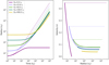 |
Fig. 1. Left: radial distance from the black hole r(t) as a function of t for λEdd = 1 and |
As expected, relativistic effects reduce radiation pressure, resulting in a deceleration of the wind under the gravitational pull of the SMBH. Indeed, it can be seen that the wind trajectories, especially the ones at smaller radii (i.e. closer to the black hole) undergo a significant velocity reduction. In the extreme case of r0 = 5 rG, the velocity drops to 0. When v = 0, relativistic effects vanish and radiation pressure is able, as in the classic case, to sustain the wind against the gravitational force, leading to a “stalling wind”. The highest final velocity is given by the case with r0 = 50.0 rG and it is ≈0.1c, which is consistent with the typical observed UFO velocities (e.g., Tombesi et al. 2011; Gofford et al. 2015).
3. Axisymmetric wind launched from an accretion disk
Let us now rewrite Eqs. (5a)–(5d) in the case of a wind launched from an accretion disc. We assume axisymmetry and a geometrically thin disc, such as in Shakura & Sunyaev (1973), orbiting with a Keplerian profile. We adopt a cylindrical coordinate system (R, ϕ, z). The set of equations is then:
 (6a)
(6a)
 (6b)
(6b)
 (6c)
(6c)
 (6d)
(6d)
 (6e)
(6e)
 (6f)
(6f)
 (6g)
(6g)
where, as in Eqs. (5a)–(5d), r, t are in units of rG, tG, θ is the angle between the incident luminosity and the direction of motion of the gas and we assume that the luminosity source is point-like. Hereafter, we indicate in bold the vectorial quantities. In the first two equations, the second term in the right-hand bracket corresponds to the gravitational attraction; l is the specific angular momentum (angular momentum per unit mass), which is a conserved quantity during the motion; r0, v0 are the starting radius and velocity, respectively. We assume that initially, the gas lies on the disk plane and the starting velocity lifts the gas above the disk, along the z coordinate, with a velocity proportional to the disc rotational velocity,  . The velocity along the ϕ coordinate is updated at each step to ensure the conservation of l. These initial conditions are rather general, and represents a good approximation of the radiatively driven wind scenario (Proga et al. 2000; Proga & Kallman 2004), as well as the magneto-hydrodynamic (MHD) scenario, in which the gas is lifted through magnetic field lines that are co-rotating with the disk (Blandford & Payne 1982; Contopoulos & Lovelace 1994; Fukumura et al. 2010, 2014; Cui & Yuan 2020).
Figure 2 shows the solutions of Eqs. (6a)–(6g) for R0 = [5.0, 15.8, 50.0, 158.1, 500.0] rG, an integration time of 106 tG, a logarithmic temporal resolution of 5 × 10⁶ steps, as in Sect. 2, λEdd = 1, and vz, 0 = vrot. For comparison, we also show the corresponding classic solutions. As expected, the highest differences are observed at smaller radii, where the velocity is higher and the relativistic effects are stronger. We present a detailed plot of the wind dynamics in Fig. A.1.
 |
Fig. 2. Wind trajectories for vz, 0 = vrot and λEdd = 1 in axisymmetric geometry. From left to right: trajectories of the wind in the z − R plane (x-axis corresponds to the radius and y-axis to the altitude from the disc plane); outflow velocity vout as a function of r (where |


Hereafter, we concentrate on the outflow velocity, defined as  , rather than on the total wind velocity
  , for a more optimal comparison of our results with observations. The velocity of the observed UFOs is primarily derived through spectroscopy, thanks to the Doppler shift of the wind absorption lines. These lines are usually described with Gaussian or Voight profiles, which means that they have an average energy and some degree of broadening. The observed wind outflow velocity, vobs, is usually derived from the average velocity, while the broadening is phenomenologically ascribed to turbulence or rotational motion within the wind.
In our model, vobs is given by the projection of vR + vz along the line of sight (LOS), while the rotational velocity, vϕ, only contributes to the broadening of the line thanks to the axisymmetry of the system. The highest vobs is given by vout, and corresponds to the case in which the LOS is parallel to vR + vz. We refer to Fukumura & Tombesi (2019) for a detailed discussion on this point. Interestingly, the authors discuss the possibility that a rotational motion of the wind around the X-ray corona is responsible for the broadening of the absorption lines, in a similar way as in the scenario discussed here.
4. Force multipliers
In the literature on accretion disc wind, the wind opacity is usually calculated analytically over a broad range of absorption lines in the UV and X-ray energy range (see e.g., Proga & Kallman 2004; Risaliti & Elvis 2010; Sim et al. 2010; Dyda & Proga 2018; Quera-Bofarull et al. 2020), obtaining so-called ‘force multipliers’. Here, we use the radiative transfer code XSTAR (Kallman & Bautista 2001). Saez & Chartas (2011) and Chartas et al. (2009) performed calculations in a similar fashion using the Cloudy photoionisation code (Ferland et al. 2017), albeit with a different formalism.
XSTAR accurately computes the transmitted spectrum ST through a gas layer, as a function of the following input quantities:
-
SI, the incident spectrum, and its integrated ionising luminosity
 in the 1−1000 Ry interval (1 Ry = 13.6 eV).
 -
r0, the distance of the gas from the central luminosity source
-
n0, the gas number density at r0
-
NH, its column density
-
α, the coefficient regulating the radial dependence of n:

-
vbroad, the gas velocity dispersion regulating the broadening of the absorption features.
The difference LI − LT (where LI, LT are the integrated luminosity of SI, ST) corresponds to the amount of radiation absorbed by the wind thanks to its opacity. This difference corresponds to a momentum Δp deposited on the wind, which can be written as  , where we introduce the new variable
  . Specifically, for a given set of initial parameters [SI, r0, n0, NH, α, vbroad] we run an XSTAR simulation and we calculate frad as:
 (7)
(7)
where E0, E1 correspond to the lower and upper energy bound and  ,
,  are the incident and transmitted flux, respectively, as functions of the frequency ν, such that
  and
and  . From a mathematical point of view, frad corresponds to a weighted average of the wind opacity. In all the cases of interest, absorption features are comprised in the energy interval between 0.1 eV and 100 keV, which we chose as E0, E1, respectively.
It is important to note that XSTAR, as well as other photoionisation codes such as Cloudy, does not allow the inclusion of a net velocity of the gas and the related relativistic effects. In order to take them into account, it is convenient to transform the spectra from the rest frame K to the wind reference frame K′, and to manipulate SI and ST, namely to shift their frequencies by a factor ψ and multiply their fluxes by ψ3 (we refer to Luminari et al. 2020 for a detailed explanation). However, since frad is calculated as a ratio between ST and SI, the transformations cancel out, so frad can be directly calculated in K without the need of any relativistic transformation.
We integrate the equation of motion in Eq. (2) for a radial interval Δr, in which a wind column density NH is enclosed, and we include the momentum Δp. The resulting equation is:
 (8)
(8)
where we also include Thompson scattering and  ,
,  correspond to the bolometric luminosity and the incident luminosity between E0 and E1, respectively. The ′ symbol indicates that the luminosities are in the K′ frame, that is,
  . It must be noted that for this equation to hold, Δr must be small enough so that r can be approximated as constant (i.e. Δr ≪ r).
We set our work within the same frame presented in Sect. 3 (axisymmetry, thin accretion disk, and the conservation of l). The complete set of equations is then:
 (9a)
(9a)
 (9b)
(9b)
 (9c)
(9c)
 (9d)
(9d)
 (9e)
(9e)
 (9f)
(9f)
 (9g)
(9g)
where, as in Sect. 3, r, t are in units of rG, tG and  ,
,  .
.
5. Initial parameters and force multipliers calculation
5.1. Model setup
Since we are primarily interested in winds from AGN accretion discs, we focus on ‘typical’ values of λEdd between 0.1 and 2.0 and a black hole mass M = 108 M⊙. However, as we show later in this section, the properties of the wind, and then the values of frad, mainly depend on λEdd, rather than on M or Lbol alone, so our results are applicable regardless of the black hole mass.
We use the bolometric corrections of Lusso et al. (2012) to obtain the 2−10 keV luminosities. We assume a simple powerlaw incident spectrum with photon index Γ = 2, consistent with the typical values observed in AGN (Piconcelli et al. 2005; Tombesi et al. 2011), to extrapolate Lion and LUX.
Regarding the properties of the wind, we concentrate on a set of initial number density log(n0/cm3) ∈ [10, 11, 12, 13] in order to match the ionisation parameters of the observed UFOs, as we discuss in the following, and the range of NH ∈ [5 × 10²², 1024] cm−2. As the starting radii, we use the same set of values given in Sects. 2 and 3: R0 ∈ [5.0, 15.8, 50.0, 158.1, 500.0] rG. In our scenario, we assume that all the luminosity comes from a point source located at the coordinate origin (R = 0, z = 0). However, we note that, observationally, the X-ray flux is usually ascribed to a hot ‘corona’, comprised within ∼10 rG from the SMBH (Chartas et al. 2012; Reis & Miller 2013; Reis et al. 2014; Kara et al. 2016; Caballero-García et al. 2020; Szanecki et al. 2020), while the UV radiation is due to the disc emissivity which, for a thin disc, has its peak at ∼20 rG (Quera-Bofarull et al. 2020). As a result, we expect that in our code the radiative contribution may not be fully modelled for R0 < 50.0 rG; however, we include the cases for R0 = 5.0, 15.8 rG, since the fate of the wind is governed primarily by v0, rather than by the radiation pressure, as we show further on.
We fix α, the exponent regulating the radial dependence of n, to 2, so that  , as expected by mass conservation for a medium expanding in a spherical geometry. Since we expect a high degree of velocity shear within the wind due to its acceleration, we use a high turbulent velocity vbroad = 3000 km s−1 to prevent line saturation. This value is consistent with those typically observed in UFOs (see e.g., Fukumura & Tombesi 2019 and references therein).
We briefly summarise here the range of input quantities of our simulations, from which we calculate a grid of frad values:
-
λEdd: we divide the interval of interest in four values, logarithmically spaced: λEdd = [0.1, 0.5, 1., 2.]
-
n0: we divide the range in logarithmic steps: log(n0/cm3) ∈ [10, 11, 12, 13]
-
r0 ∈ [5.0, 15.8, 50.0, 158.1, 500.0] rG
-
NH: we span the range [5 × 10²², 1024] cm−2 with steps of 5 × 1022 cm−2
We compute the geometrical thickness of the wind to check whether the Δr ≪ r condition in Eq. (8) is met. The results plotted in Fig. B.1 (first three panels) in the appendix show that ΔR/R0 < 1 for all cases. The only exception is for R0 = 5 rG, log(n0/cm3) = 10, when the column density is very high (NH > 7 × 1023 cm−2). However, as we discuss further on, the properties of the wind are quite independent from NH, and we focus on the typical UFO value of NH = 1023 cm−2 (Tombesi et al. 2011) in most cases. In the last panel of Fig. B.1, we show the ionisation parameter ξ(r), defined as  , for λEdd = 1.0, 0.1. This parameter is of great importance since the absorption structure of the wind, and thus the values of frad, mainly depends on it. Our range of ξ, from ∼100 to ∼106, agrees well with the broad population of UFOs and warm absorbers (see e.g., Laha et al. 2014, 2016; Serafinelli et al. 2019); this, in turn, justifies our range of log(n0). Moreover, our values for log(n0) are in agreement with those commonly estimated for the broad line region (BLR) and for UV and X-ray outflows (see e.g., Elvis 2000; Schurch & Done 2007; Saez & Chartas 2011; Netzer 2013). Finally, in Fig. B.2 we show the values of frad as a function of the wind parameters.
5.2. Impact of the initial parameters on the wind dynamics
We solve the system of Eqs. (9a)–(9g) for the whole grid of initial parameters for an integration time of 106 tG, the same temporal resolution of Sect. 2 and using a set of vz,0 ∈ [1.0, 10−1, 10−2, 10−3]vrot. For a complete discussion of the results, we first analyse the impact of the different parameters. To characterise the wind dynamics, we define a wind successfully launched if it has a positive (outbound) velocity at the end of the integration time, t = t1, and we compute its terminal velocity as  .
.
Here, λEdd and vz, 0 are the dominant parameters since they regulate the amount of radiation pressure and the initial velocity of the wind. When vz, 0 = vrot, the high initial velocity allows the wind to be successfully launched for any value of λEdd (albeit reaching different vt). For vz,0 = 10−1, 10−2, 10−3 vrot, instead, the impact of the initial velocity itself to the wind evolution is almost negligible, and the different solutions are indistinguishable between them. However, vz, 0 lifts the gas above the disk, displacing it from its equilibrium radius and exposing it to the radiation pressure. The fate of the wind then depends on λEdd and, secondarily, on R0, but it is unaffected by the exact value of vz, 0. We plot in Fig. 3 the failed wind region (i.e. the radius up to which the wind cannot be succesfully launched) as a function of λEdd, for different vz, 0. For vz, 0 = vrot, the wind is always successful. Then, the failed region increases for decreasing vz, 0, and becomes quite constant for vz,0 ≤ 10−1 vrot. Please note that in this figure we do not take into account wind opacity (i.e. we use the same treatment of Sect. 3) due to the long computational times required. However, the overall behaviour of vz, 0 is similar. For simplicity going forward, we concentrate only on vz,0 = 10−2, 1.0] vrot. We note that vz, 0 = vrot represents a remarkably high starting velocity, which could be justified only under certain particular physical conditions (see discussion in Sect. 7) and is significantly higher from the velocities commonly assumed in the literature, which are closer to the vz,0 = 10−2 vrot case (see e.g., Proga et al. 2000; Nomura et al. 2016, 2020). As we will detail in the following, we run the simulations using this starting value as a case study in order to set an upper bound for the wind velocities that can be reached through radiative pressure, once they have been corrected for relativistic effects.
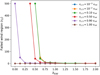 |
Fig. 3. Failed wind region as a function of λEdd = for different vz, 0 (colour coding, see legend). It can be seen that for vz,0 ≤ 10−1 vrot the region becomes quite constant, since the wind dynamics no longer depends on the value of vz, 0. |
In what concerns n0, it can give rise to differences in vt of up to 0.05c, but it generally does not affect the overall behaviour of the wind. Since frad is always roughly directly proportional to the column density, the wind solutions are also quite independent from NH because these two terms balance each other in the first term on the right-hand side of Eqs. (9a) and (9b). We note that this trend also holds for optically thick winds. In facts, for column densities of  cm−2, the line opacity grows equally or less than linearly with NH (Tombesi et al. 2011), and so the frad/NH term in Eqs. (9a) and (9b) do not contribute any more than for the optically thin wind. We refer to Appendix C for further discussions on n0, NH. From this point on, we focus on log(n0/cm3) = 11, NH = 1023 cm−2, unless stated otherwise.
6. Results
To examine the wind behaviour, we plot in Fig. 4 the trajectories in the R − z plane for λEdd = 0.1, 1.0 (left and right panels, respectively). Hereafter, we convert the distance from the black hole (x-axis) from rG to pc assuming M = 108 M⊙. As discussed in Sect. 5.2, the dominant parameter in the wind motion is vz, 0: for vz, 0 = vrot (solid lines), the wind is always successful, whereas for vz,0 = 10−2 vrot (dashed lines), it can be launched only for λEdd = 1.0 and R0 > 5 rG. In Fig. 4 and in the following, a truncated trajectory corresponds to a failed wind since we interrupt the numerical integration when the gas falls back to the disk plane. Classic and relativistic trajectories (represented with bold and thin lines, respectively) are almost indistinguishable; however, as we will see in the following, their velocities are rather different.
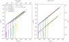 |
Fig. 4. Trajectories of the wind in the z − R plane (y and x axis, respectively) for λEdd = 0.1, 1.0 (left and right panel, respectively). Solid (dashed) lines correspond to vz,0 = vrot(10−2 vrot). Thick and thin lines refer to the relativistic and classic (i.e. non-relativistic) treatment. Distances are reported both in units of rG and pc, where the latter are calculated assuming M = 108 M⊙. |
In Fig. 5 we show a comparison between the velocities in the relativistic and in the classic treatments (bold and thin lines, respectively) as a function of t, for λEdd = 0.1, 1.0 (left and right panel, respectively). Purple, light-blue, and green lines correspond to R0 = 5.0, 50.0, 500.0 rG, respectively. Solid(dashed) lines correspond to v0 = 1.0(= 10−2 vrot). The impact of relativistic effects is remarkable, especially in the highest velocity cases. The maximum vt drops from ≈0.6 to less than 0.3c when taking into account the reduction of radiative pressure due to special relativity effects. We also note that in most of the cases, the wind attains its terminal velocity within 104 tG (corresponding to 0.1 yr, i.e. roughly a month, for M = 108 M⊙). For R0 = 5 rG, this time is reduced to 103 tG (10−2 yr, i.e. a few days). For comparison, we indicate the times corresponding to one day and one month with vertical dotted lines.
 |
Fig. 5. Velocity of the wind as a function of tG for λEdd = 0.1, 1.0 (left and right panel, respectively). Line styles as in Fig. 4. Times are converted from tG to yr assuming M = 108 M⊙. |
In Fig. 6 we show the velocity of the wind as a function of the distance from the black hole. Line styles are as in Fig. 5. To give an idea of the dimensions of the accretion disc-torus system, we also indicate the typical distance at which BLR are observed and the dust sublimation radius, as a proxy of the inner boundary of the torus. We chose 0.01 pc as the BLR inner radius and 0.5 pc as the dust sublimation radius, which marks the boundary between the BLR and the torus (Coffey et al. 2014; Różańska et al. 2014; Adhikari et al. 2016; Sturm et al. 2018; Czerny 2019).
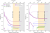 |
Fig. 6. Velocity versus distance from the black hole for λEdd = 0.1, 1.0 (left and right panel, respectively). Line styles as in Fig. 4. Distances are converted from rG to pc assuming M = 108 M⊙. |
For a detailed analysis of the wind dynamics, we show the case for λEdd = 1, vz, 0 = vrot in Fig. D.1.
7. Discussion
To illustrate the overall behaviour of the wind, we plot (Fig. 7) vt as a function of R0 for vz, 0 = 10−2, 1.0 vrot (left and right panel). We also plot the vt obtained in the classic case with dashed lines. The null values indicate an unsuccessful wind. In order for the wind to attain the typical velocities of UFOs, that is, ≳0.1c (see e.g., Fiore et al. 2017 for a set of values from the literature), either the luminosity must be very high (λEdd ≥ 1.0) or the initial velocity, vz, 0, must be comparable to the rotational velocity, vrot.
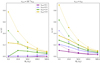 |
Fig. 7. Terminal velocities, vt, as functions of R0 for different values of λEdd (colour coding). Solid lines refer to the relativistic treatment, dashed to the classic (non-relativistic) one. Left panel: vz,0 = 10−2 vrot; right panel: vz, 0 = vrot. |
In Fig. 8 we plot vt as a function of ξ0 (which is a monotonically decreasing function of R0) in the densest and in the lightest cases, that is, log(n0/cm3) = 10 and = 13 for λEdd = 0.1 and = 1.0 (left and right panels, respectively). Generally, vt is found to be a monotonically increasing function of ξ (see e.g., Tombesi et al. 2013). Interestingly, this behaviour can be reproduced only with vz, 0 ∝ vrot.
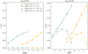 |
Fig. 8. Terminal velocities, vt, as functions of ξ0 for log(n0) = 10, 13 (in units of cm−3; yellow and gray lines, respectively). Solid and dashed lines refer to vz, 0 = vrot and = 10−2 vrot, respectively. Left panel: λEdd = 0.1; right panel: = 1.0. |
We now compare our results with UFOs from the literature. Our goal is to establish whether the observed UFO velocities can be reproduced within our radiative driving framework. To do so, we consider two different limiting velocities emerging from our results. The first one is the terminal velocity, vt, which is almost reached by the wind after a very short time and is, thus, the most likely to be observed. The second one is the maximum velocity reached by the wind, vmax, which is associated with the short-living, initial phases of the wind motion (see Figs. 5 and 6), and, hence, represents an upper limit of the observable velocity. Since we are interested in the highest possible velocities, we focus on the vz, 0 = vrot cases.
We compute the highest values of vt, vmax as a function of λEdd for R0 ≥ 50.0 rG, which represents a lower bound for the launching radius of the observed UFOs (see discussion in Sect. 2). We plot the results in Fig. 9, denoting with dark orange and blue the regions below the curves of vt, vmax, respectively. These regions correspond to the allowed velocity ranges.
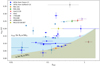 |
Fig. 9. Comparison between UFO velocities from the literature (dots and squares) and the results of the present work as a function of λEdd. The theoretical limit according to the terminal velocity, vt, for R0 ≥ 50 rG corresponds to the orange shaded area. The limit according to the maximum (but short-lived) velocity, vmax, corresponds to the light-blue area. See Appendix E for a description of the sample and the related references. |
We show with different symbols (see legend) the location of several UFOs reported in the literature (see Appendix E for references on the single sources). Interestingly, many points lie above the vt (orange) allowed region, and many also above the vmax (blue) region. Such high velocities, which can be hardly explained within our radiative driving model, may lend support to other launching mechanisms. As discussed in Sect. 5.2, vz, 0 = vrot represents an upper bound of the expected launching velocities for a radiatively-driven wind. Lower, physically-motivated vz, 0 would result in even lower limiting velocities than those reported in Fig. 9, thus strengthening our conclusion that radiative driving, once corrected for special relativity effects, is not sufficient to produce the observed UFO velocity distribution.
In particular, we signal the possibility of a magnetocentrifugal acceleration mechanism, which is capable of driving the wind up to very high terminal velocities. Typical values are close to between one and three times the rotational velocity at the wind launching radius, R0 (Fukumura et al. 2010, 2014; Tombesi et al. 2013; Cui & Yuan 2020). For R0 = 50 rG, this corresponds to terminal velocities between 0.14 and 0.42c, thus easily accounting for the observed UFO velocities.
We outline two interesting implications of our results. Several observations show the simultaneous presence in AGN X-ray spectra of fast absorbers with comparable vout ∼ 0.1−0.2c and orders of magnitude differences between their ξ (Longinotti et al. 2015; Serafinelli et al. 2019; Reeves et al. 2020). This evidence can be easily explained within our model. The weak dependence of the outflow solutions from n0 indicates that different wind elements can be launched with similar velocity (and column density) but rather different ionisation parameters, as shown in Fig. 8. This, in turn, is due to the sub-dominant contribution of the force multipliers (and then of the line driving) with respect to Thompson scattering, as outlined also in Dannen et al. (2019).
Secondly, failed winds (FW) are a natural outcome in any radiative driven scenario, and we expect their presence to be ubiquitous if the radiation is the main driver. In fact, in our analysis we show that successful winds can be launched only through very high launching velocities (vz, 0 ∝ vrot) or extreme luminosities λEdd (≳1). However, many hosting UFOs have λEdd ∼ 0.1 (see Fig. 9), and such high vz, 0 are very difficult to justify in the framework of a steady-state accretion disc, unless postulating a ‘kick velocity’ through hydrodynamic instabilities (see e.g., Janiuk & Czerny 2011 and references therein), disc magnetic reconnection (Di Matteo 1998; Ergun et al. 2020; Ripperda et al. 2020) or, again, resorting to a large scale MHD-driven outflow (see Yuan et al. 2015 for numerical simulations). Within the dynamics of the accretion-ejection system, we expect the FW to act as a shield for the gas launched at higher R0, possibly regulating its ionisation status and observational properties (Giustini & Proga 2019a,b). However, we note that the effectiveness of FW in favouring the launching of more distant layers of gas has not been proven yet (Higginbottom et al. 2014; see discussion in Zappacosta et al. 2020 and references therein). FW are confined into a narrow equatorial region (i.e. their z height is ≪ than the radial coordinate, r, see Fig. 4) since the gravitational attraction prevents them from reaching high altitudes before bouncing back to the accretion disc, making them particularly difficult to observe. A careful modelisation of the wind duty cycle and of the disc region is needed in order to further shed light on this topic.
Finally, we note that our results are also robust with regard to the case of X-ray luminosity variability, as has been observed in several sources (Nardini et al. 2015; Parker et al. 2017). As discussed above, for the typical UFO ionisation degrees most of the radiative pressure is channelled through Thompson scattering, rather than line pressure. Thus, the driving luminosity is Lbol (expressed here as λEdd), which significantly varies in AGN only on timescales larger than tens of years, rather than the X-ray luminosity (expressed through λUX).
8. Conclusion
Special relativity effects strongly reduce the radiative pressure exerted on fast moving clumps of gas, as in the case of UFOs from accretion discs, as well as BAL winds. In this work, we carry out an extensive analysis of the radiative driving for a disc wind accounting for these effects. Our main findings can be summarised as follows:
-
The dynamics of the wind is primarily governed by the AGN luminosity and the launching velocity vz, 0. For high luminosity, λEdd = 1.0, the wind is successfully launched independently from vz, 0, while for λEdd = 0.1 a higher vz, 0, of the order of the disc rotational velocity, is required in order to overcome the gravitational attraction from the central black hole (see Fig. 4).
-
Shortly after the launch of the wind (between one day and one month, depending on R0), the wind attains a roughly constant velocity, vt, which is conserved until the end of the integration time (106 tG, i.e. 10 yr for a black hole mass of 108 M⊙). After about one month, the wind reaches BLR-like distances, possibly suggesting an interaction with the gas in the BLR orbiting above the accretion disc.
-
The inclusion of special relativity effects reduces the radiative pressure exerted on the wind. This, in turn, leads to remarkably lower vt with respect to the classical treatment, up to 50% less for winds launched at the smallest R0. Within the relativistic treatment, we find an upper limit of vt = 0.15c for the highest luminosity case (λEdd = 1.0) and a launching radius of ≥50 rG, which is in agreement with the observed UFO locations.
-
Interestingly, we find that most of the UFO velocities from the literature cannot be reproduced within our radiative-driving scenario. For the majority of the sources, which have λEdd between 0.03 and 1, the luminosity is too low to reproduce the observed vout. This evidence suggests that other acceleration mechanisms are at play. In particular, we suggest the possibility of magnetic driving, which could easily account for the observed vout.
Acknowledgments
We thank the referee for the valuable comments that helped improve the paper and Manuela Bischetti for discussions on the UFO host galaxies. AL deeply thanks all the staff at the Harvard & Smithsonian Center for Astrophysics for their warm welcome during the time spent there. AL, EP, FT, LZ acknowledge financial support under ASI-INAF contract 2017-14-H.0. EP, FF acknowledge support from PRIN MIUR project “Black Hole winds and the Baryon Life Cycle of Galaxies: the stone-guest at the galaxy evolution supper”, contract #2017PH3WAT.
References
- Adhikari, T. P., Różańska, A., Czerny, B., et al. 2016, ApJ, 831, 68 [Google Scholar]
- Bentz, M. C., & Manne-Nicholas, E. 2018, ApJ, 864, 146 [NASA ADS] [CrossRef] [EDP Sciences] [Google Scholar]
- Bischetti, M., Piconcelli, E., Feruglio, C., et al. 2019, A&A, 628, A118 [Google Scholar]
- Blandford, R. D., & Payne, D. G. 1982, MNRAS, 199, 883 [NASA ADS] [CrossRef] [Google Scholar]
- Braito, V., Reeves, J. N., Matzeu, G. A., et al. 2018, MNRAS, 479, 3592 [Google Scholar]
- Bruni, G., Piconcelli, E., Misawa, T., et al. 2019, A&A, 630, A111 [NASA ADS] [CrossRef] [EDP Sciences] [Google Scholar]
- Caballero-García, M. D., Papadakis, I. E., Dovčiak, M., et al. 2020, MNRAS, 498, 3184 [CrossRef] [Google Scholar]
- Caglar, T., Burtscher, L., Brandl, B., et al. 2020, A&A, 634, A114 [CrossRef] [EDP Sciences] [Google Scholar]
- Chartas, G., Saez, C., Brandt, W. N., et al. 2009, ApJ, 706, 644 [Google Scholar]
- Chartas, G., Kochanek, C. S., Dai, X., et al. 2012, ApJ, 757, 137 [NASA ADS] [CrossRef] [Google Scholar]
- Chatterjee, R., Marscher, A. P., Jorstad, S. G., et al. 2011, ApJ, 734, 43 [Google Scholar]
- Coffey, D., Longinotti, A. L., Rodríguez-Ardila, A., et al. 2014, MNRAS, 443, 1788 [NASA ADS] [CrossRef] [Google Scholar]
- Czerny, B. 2019, Open Astron., 28, 200 [Google Scholar]
- Contopoulos, J., & Lovelace, R. V. E. 1994, ApJ, 429, 139 [NASA ADS] [CrossRef] [Google Scholar]
- Cui, C., & Yuan, F. 2020, ApJ, 890, 81 [Google Scholar]
- Dannen, R. C., Proga, D., Kallman, T. R., et al. 2019, ApJ, 882, 99 [Google Scholar]
- Di Matteo, T. 1998, MNRAS, 299, L15 [NASA ADS] [CrossRef] [Google Scholar]
- Di Matteo, T., Springel, V., & Hernquist, L. 2005, Nature, 433, 604 [NASA ADS] [CrossRef] [PubMed] [Google Scholar]
- Dyda, S., & Proga, D. 2018, MNRAS, 481, 5263 [Google Scholar]
- Elvis, M. 2000, ApJ, 545, 63 [NASA ADS] [CrossRef] [Google Scholar]
- Ergun, R. E., Ahmadi, N., Kromyda, L., et al. 2020, ApJ, 898, 154 [Google Scholar]
- Ferland, G. J., Chatzikos, M., Guzmán, F., et al. 2017, Rev. Mex. Astron. Astrofis., 53, 385 [NASA ADS] [Google Scholar]
- Feruglio, C., Fiore, F., Carniani, S., et al. 2015, A&A, 583, A99 [NASA ADS] [CrossRef] [EDP Sciences] [Google Scholar]
- Fiore, F., Feruglio, C., Shankar, F., et al. 2017, A&A, 601, A143 [NASA ADS] [CrossRef] [EDP Sciences] [Google Scholar]
- Fukumura, K., & Tombesi, F. 2019, ApJ, 885, L38 [Google Scholar]
- Fukumura, K., Kazanas, D., Contopoulos, I., et al. 2010, ApJ, 715, 636 [NASA ADS] [CrossRef] [Google Scholar]
- Fukumura, K., Tombesi, F., Kazanas, D., et al. 2014, ApJ, 780, 120 [Google Scholar]
- Gaspari, M., Melioli, C., Brighenti, F., et al. 2011, MNRAS, 411, 349 [NASA ADS] [CrossRef] [Google Scholar]
- Gofford, J., Reeves, J. N., McLaughlin, D. E., et al. 2015, MNRAS, 451, 4169 [Google Scholar]
- Giustini, M., & Proga, D. 2019a, A&A, 630, A94 [NASA ADS] [CrossRef] [EDP Sciences] [Google Scholar]
- Giustini, M., & Proga, D. 2019b, Proc. IAU, 15, 82 [CrossRef] [Google Scholar]
- Hagino, K., Odaka, H., Done, C., et al. 2015, MNRAS, 446, 663 [Google Scholar]
- Hamann, F., Chartas, G., Reeves, J., et al. 2018, MNRAS, 476, 943 [NASA ADS] [CrossRef] [Google Scholar]
- Higginbottom, N., Proga, D., Knigge, C., et al. 2014, ApJ, 789, 19 [Google Scholar]
- Hopkins, P. F., & Elvis, M. 2010, MNRAS, 401, 7 [NASA ADS] [CrossRef] [Google Scholar]
- Janiuk, A., & Czerny, B. 2011, MNRAS, 414, 2186 [Google Scholar]
- Kallman, T., & Bautista, M. 2001, ApJS, 133, 221 [NASA ADS] [CrossRef] [Google Scholar]
- Kara, E., Alston, W. N., Fabian, A. C., et al. 2016, MNRAS, 462, 511 [Google Scholar]
- Kelly, B. C., & Bechtold, J. 2007, ApJS, 168, 1 [NASA ADS] [CrossRef] [Google Scholar]
- King, A., & Pounds, K. 2015, ARA&A, 53, 115 [Google Scholar]
- Kormendy, J., & Ho, L. C. 2013, ARA&A, 51, 511 [Google Scholar]
- Laha, S., Guainazzi, M., Dewangan, G. C., et al. 2014, MNRAS, 441, 2613 [Google Scholar]
- Laha, S., Guainazzi, M., Chakravorty, S., et al. 2016, MNRAS, 457, 3896 [NASA ADS] [CrossRef] [Google Scholar]
- Laha, S., Reynolds, C. S., Reeves, J., et al. 2020, Nature Astron., 5, 13 [Google Scholar]
- Laurenti, M., Luminari, A., Tombesi, F., et al. 2021, A&A, 645, A118 [CrossRef] [EDP Sciences] [Google Scholar]
- Longinotti, A. L., Krongold, Y., Guainazzi, M., et al. 2015, ApJ, 813, L39 [NASA ADS] [CrossRef] [EDP Sciences] [Google Scholar]
- Luminari, A., Tombesi, F., Piconcelli, E., et al. 2020, A&A, 633, A55 [Google Scholar]
- Lusso, E., Comastri, A., Simmons, B. D., et al. 2012, MNRAS, 425, 623 [NASA ADS] [CrossRef] [Google Scholar]
- Matthews, J. H., Knigge, C., Higginbottom, N., et al. 2020, MNRAS, 492, 5540 [Google Scholar]
- Nardini, E., & Zubovas, K. 2018, MNRAS, 478, 2274 [Google Scholar]
- Nardini, E., Reeves, J. N., Gofford, J., et al. 2015, Science, 347, 860 [Google Scholar]
- Netzer, H. 2013, The Physics and Evolution of Active Galactic Nuclei (Cambridge: Cambridge University Press) [CrossRef] [Google Scholar]
- Nomura, M., Ohsuga, K., Takahashi, H. R., et al. 2016, PASJ, 68, 16 [NASA ADS] [CrossRef] [Google Scholar]
- Nomura, M., Ohsuga, K., & Done, C. 2020, MNRAS, 494, 3616 [Google Scholar]
- Onori, F., Ricci, F., La Franca, F., et al. 2017, MNRAS, 468, L97 [Google Scholar]
- Parker, M. L., Pinto, C., Fabian, A. C., et al. 2017, Nature, 543, 83 [NASA ADS] [CrossRef] [Google Scholar]
- Peterson, B. M., Ferrarese, L., Gilbert, K. M., et al. 2004, ApJ, 613, 682 [Google Scholar]
- Piconcelli, E., Jimenez-Bailón, E., Guainazzi, M., et al. 2005, A&A, 432, 15 [NASA ADS] [CrossRef] [EDP Sciences] [Google Scholar]
- Proga, D., & Kallman, T. R. 2004, ApJ, 616, 688 [Google Scholar]
- Proga, D., Stone, J. M., & Kallman, T. R. 2000, ApJ, 543, 686 [NASA ADS] [CrossRef] [Google Scholar]
- Quera-Bofarull, A., Done, C., Lacey, C., et al. 2020, MNRAS, 495, 402 [Google Scholar]
- Reeves, J. N., & Braito, V. 2019, ApJ, 884, 80 [Google Scholar]
- Reeves, J. N., Braito, V., Chartas, G., et al. 2020, ApJ, 895, 37 [Google Scholar]
- Reis, R. C., & Miller, J. M. 2013, ApJ, 769, L7 [Google Scholar]
- Reis, R. C., Reynolds, M. T., Miller, J. M., et al. 2014, Nature, 507, 207 [NASA ADS] [CrossRef] [EDP Sciences] [Google Scholar]
- Ricci, F., La Franca, F., Onori, F., et al. 2017a, A&A, 598, A51 [Google Scholar]
- Ricci, F., La Franca, F., Marconi, A., et al. 2017b, MNRAS, 471, L41 [NASA ADS] [CrossRef] [Google Scholar]
- Ripperda, B., Bacchini, F., & Philippov, A. A. 2020, ApJ, 900, 100 [Google Scholar]
- Risaliti, G., & Elvis, M. 2010, A&A, 516, A89 [NASA ADS] [CrossRef] [EDP Sciences] [Google Scholar]
- Różańska, A., Nikołajuk, M., Czerny, B., et al. 2014, New Astron., 28, 70 [NASA ADS] [CrossRef] [Google Scholar]
- Rybicki, G. B., & Lightman, A. P. 1986, Radiative Processes in Astrophysics (Weinheim: Wiley-VCH) [Google Scholar]
- Saez, C., & Chartas, G. 2011, ApJ, 737, 91 [Google Scholar]
- Saturni, F. G., Bischetti, M., Piconcelli, E., et al. 2018, A&A, 617, A118 [NASA ADS] [CrossRef] [EDP Sciences] [Google Scholar]
- Schurch, N. J., & Done, C. 2007, MNRAS, 381, 1413 [Google Scholar]
- Shakura, N. I., & Sunyaev, R. A. 1973, A&A, 500, 33 [NASA ADS] [Google Scholar]
- Serafinelli, R., Tombesi, F., Vagnetti, F., et al. 2019, A&A, 627, A121 [NASA ADS] [CrossRef] [EDP Sciences] [Google Scholar]
- Sim, S. A., Proga, D., Miller, L., et al. 2010, MNRAS, 408, 1396 [Google Scholar]
- Smith, R. N., Tombesi, F., Veilleux, S., et al. 2019, ApJ, 887, 69 [NASA ADS] [CrossRef] [Google Scholar]
- Sturm, E., Dexter, J., Pfuhl, O., et al. 2018, Nature, 563, 657 [Google Scholar]
- Szanecki, M., Niedźwiecki, A., Done, C., et al. 2020, A&A, 641, A89 [CrossRef] [EDP Sciences] [Google Scholar]
- Tilton, E. M., & Shull, J. M. 2013, ApJ, 774, 67 [NASA ADS] [CrossRef] [Google Scholar]
- Tombesi, F., Cappi, M., Reeves, J. N., et al. 2011, ApJ, 742, 44 [Google Scholar]
- Tombesi, F., Cappi, M., Reeves, J. N., et al. 2012, MNRAS, 422, L1 [NASA ADS] [CrossRef] [Google Scholar]
- Tombesi, F., Cappi, M., Reeves, J. N., et al. 2013, MNRAS, 430, 1102 [Google Scholar]
- Tombesi, F., Meléndez, M., Veilleux, S., et al. 2015, Nature, 519, 436 [Google Scholar]
- Vestergaard, M., & Peterson, B. M. 2006, ApJ, 641, 689 [Google Scholar]
- Yuan, F., Gan, Z., Narayan, R., et al. 2015, ApJ, 804, 101 [NASA ADS] [CrossRef] [Google Scholar]
- Zappacosta, L., Piconcelli, E., Giustini, M., et al. 2020, A&A, 635, L5 [NASA ADS] [CrossRef] [EDP Sciences] [Google Scholar]
Appendix A: Three-dimensional wind
We show in Fig. A.1 a detailed analysis of the wind trajectories for the preliminary three-dimensional model presented in Sect. 3.
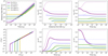 |
Fig. A.1. Wind trajectories for vz, 0 = vrot and λEdd = 1. From top to bottom and left to right: distance r from the BH (where |


Appendix B: Geometrical and physical properties of the wind
We show in Fig. B.1 (first three panels) the geometrical thickness of the wind. With our density profile  (see Sect. 5), the upper limit for the column density corresponds to NH, max = n0 r0. For all the values of n0, r0 in this paper, NH, max > 1024 cm−2. The only exception is for n0 = 1010 cm−3, r0 = 5 rG (first panel, blue line), for which NH, max = 7.4 × 1023 cm−2. In the last panel of Fig. B.1 we plot ξ(r) for λEdd = 0.1, 1.0. Figure B.2 shows frad as a function of NH, for different R0 (colour coding) and log(n0/cm3) = 10, 11, 12, 13 (from left to right). From top to bottom, λEdd = 0.1, 0.5, 1.0, 2.0.
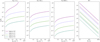 |
Fig. B.1. First three panels: geometrical thickness of the wind as a function of NH for log(n0) = 10, 11, 12, 13 (in units of cm−3, colour coding) and increasing R0 (from left to right). Last panel: ionisation parameter as a function of R0 for different log(n0) (colour coding) and λEdd = 0.1, 1.0 (dashed and solid lines, respectively). |
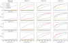 |
Fig. B.2. Values of frad as functions of NH for log(n0) = 10, 11, 12, 13 (in units of cm−3, from left to right) and λEdd = 0.1, 0.5, 1.0, 2.0 (from top to bottom). |
Appendix C: Dependence of the wind dynamics on n0, NH
To give an idea of the impact of n0 on the wind dynamics, we show in Fig. C.1 the terminal velocity vt as a function of R0 for different n0 (colour coding). From left to right, λEdd = 0.1, 0.5, 1.0, 2.0. Top (bottom) row refers to vz, 0 = vrot(vz,0 = 10−2 vrot). Here, vt is similar for any value of n0, except for vz, 0 = 0.01 vrot and λEdd = 0.5, 1.0, where the initial velocity is low enough (and the luminosity is not too low nor too high) so that different frad values can give rise to different wind behaviours.
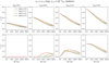 |
Fig. C.1. Terminal velocity of the wind for log(n0) = 10, 11, 12, 13 (in units of cm−3, colour-coding) and for different luminosities (from left to rightλEdd = 0.1, 0.5, 1.0, 2.0). Top (bottom) panel: vz, 0 = vrot(vz,0 = 10−2 vrot). For simplicity, we fix NH = 1023 cm−2. |
Similarly, in Fig. C.2 we plot vt for log(n0/cm3) = 10, 13 for the lower and upper values of NH (5 × 10²² and 1024 cm−2). It can be seen that the overall dynamics of the wind is weakly sensitive to NH.
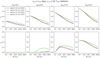 |
Fig. C.2. Terminal velocity of the wind for log(n0) = 10, 13 (in units of cm−3, purple and green lines) and NH = 5 × 10²² and = 1024 (in units of cm−2, solid and dashed lines). Top (bottom) panel: vz, 0 = vrot(vz,0 = 10−2 vrot). |
Appendix D: Results
We present in Fig. D.1 a detailed analysis of the wind dynamics for λEdd = 1, vz, 0 = vrot, log(n0/cm3) = 11, NH = 1023 cm−2 and taking into account the wind opacity (Sect. 4).
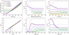 |
Fig. D.1. Wind solutions in the relativistic and classic cases (solid and dashed lines, respectively) for λEdd = 1, vz, 0 = vrot and taking into account the wind opacity. Meaning of the panels as in Fig. A.1. |
Appendix E: Notes on UFOs sources from literature
We show in Table E.1 the properties of the sources plotted in Fig. 9. The sample is composed of three main groups. The first one is taken from the Tombesi et al. (2011) sample, with the updated Lbol from Fiore et al. (2017), while the second one is from Gofford et al. (2015). The third one comprises the sources reported in Fiore et al. (2017) and not previously reported in Tombesi et al. (2011), together with other individually-reported UFOs published from 2017 on for which robust estimates of both λEdd and vout are available. Where possible, the black hole mass M and the AGN bolometric luminosity Lbol have been updated with recent works, listed in the last column.
Sources plotted in Fig. 9.
All Tables
All Figures
|
Fig. 1. Left: radial distance from the black hole r(t) as a function of t for λEdd = 1 and |
| In the text | |
|
Fig. 2. Wind trajectories for vz, 0 = vrot and λEdd = 1 in axisymmetric geometry. From left to right: trajectories of the wind in the z − R plane (x-axis corresponds to the radius and y-axis to the altitude from the disc plane); outflow velocity vout as a function of r (where |
| In the text | |
|
Fig. 3. Failed wind region as a function of λEdd = for different vz, 0 (colour coding, see legend). It can be seen that for vz,0 ≤ 10−1 vrot the region becomes quite constant, since the wind dynamics no longer depends on the value of vz, 0. |
| In the text | |
|
Fig. 4. Trajectories of the wind in the z − R plane (y and x axis, respectively) for λEdd = 0.1, 1.0 (left and right panel, respectively). Solid (dashed) lines correspond to vz,0 = vrot(10−2 vrot). Thick and thin lines refer to the relativistic and classic (i.e. non-relativistic) treatment. Distances are reported both in units of rG and pc, where the latter are calculated assuming M = 108 M⊙. |
| In the text | |
|
Fig. 5. Velocity of the wind as a function of tG for λEdd = 0.1, 1.0 (left and right panel, respectively). Line styles as in Fig. 4. Times are converted from tG to yr assuming M = 108 M⊙. |
| In the text | |
|
Fig. 6. Velocity versus distance from the black hole for λEdd = 0.1, 1.0 (left and right panel, respectively). Line styles as in Fig. 4. Distances are converted from rG to pc assuming M = 108 M⊙. |
| In the text | |
|
Fig. 7. Terminal velocities, vt, as functions of R0 for different values of λEdd (colour coding). Solid lines refer to the relativistic treatment, dashed to the classic (non-relativistic) one. Left panel: vz,0 = 10−2 vrot; right panel: vz, 0 = vrot. |
| In the text | |
|
Fig. 8. Terminal velocities, vt, as functions of ξ0 for log(n0) = 10, 13 (in units of cm−3; yellow and gray lines, respectively). Solid and dashed lines refer to vz, 0 = vrot and = 10−2 vrot, respectively. Left panel: λEdd = 0.1; right panel: = 1.0. |
| In the text | |
|
Fig. 9. Comparison between UFO velocities from the literature (dots and squares) and the results of the present work as a function of λEdd. The theoretical limit according to the terminal velocity, vt, for R0 ≥ 50 rG corresponds to the orange shaded area. The limit according to the maximum (but short-lived) velocity, vmax, corresponds to the light-blue area. See Appendix E for a description of the sample and the related references. |
| In the text | |
|
Fig. A.1. Wind trajectories for vz, 0 = vrot and λEdd = 1. From top to bottom and left to right: distance r from the BH (where |
| In the text | |
|
Fig. B.1. First three panels: geometrical thickness of the wind as a function of NH for log(n0) = 10, 11, 12, 13 (in units of cm−3, colour coding) and increasing R0 (from left to right). Last panel: ionisation parameter as a function of R0 for different log(n0) (colour coding) and λEdd = 0.1, 1.0 (dashed and solid lines, respectively). |
| In the text | |
|
Fig. B.2. Values of frad as functions of NH for log(n0) = 10, 11, 12, 13 (in units of cm−3, from left to right) and λEdd = 0.1, 0.5, 1.0, 2.0 (from top to bottom). |
| In the text | |
|
Fig. C.1. Terminal velocity of the wind for log(n0) = 10, 11, 12, 13 (in units of cm−3, colour-coding) and for different luminosities (from left to rightλEdd = 0.1, 0.5, 1.0, 2.0). Top (bottom) panel: vz, 0 = vrot(vz,0 = 10−2 vrot). For simplicity, we fix NH = 1023 cm−2. |
| In the text | |
|
Fig. C.2. Terminal velocity of the wind for log(n0) = 10, 13 (in units of cm−3, purple and green lines) and NH = 5 × 10²² and = 1024 (in units of cm−2, solid and dashed lines). Top (bottom) panel: vz, 0 = vrot(vz,0 = 10−2 vrot). |
| In the text | |
|
Fig. D.1. Wind solutions in the relativistic and classic cases (solid and dashed lines, respectively) for λEdd = 1, vz, 0 = vrot and taking into account the wind opacity. Meaning of the panels as in Fig. A.1. |
| In the text | |
Current usage metrics show cumulative count of Article Views (full-text article views including HTML views, PDF and ePub downloads, according to the available data) and Abstracts Views on Vision4Press platform.
Data correspond to usage on the plateform after 2015. The current usage metrics is available 48-96 hours after online publication and is updated daily on week days.
Initial download of the metrics may take a while.