© The Authors 2023

1. Introduction

At the center of virtually every galaxy, there is a supermassive black hole (SMBH) whose mass lies in the 10⁶ − 10⁹ M_⊙ range (where M_⊙ indicates solar masses). Some of these objects are active: gravitationally accreting material around them, they emit electromagnetic radiation whose luminosity can be even higher than that emitted by all the stars of the host galaxy. These objects are called active galactic nuclei (AGNs).

Radiation from AGNs spans the entire electromagnetic spectrum, from the radio up to the gamma-ray regime. In particular, the study of the absorption and emission lines in the X-ray band of several AGNs revealed layers of ionized plasma nearby the central SMBH (see Pounds et al. 2003; Cappi et al. 2009). Ultrafast outflows (UFOs) are powerful ejections of material that are launched from the accretion disk with mildly relativistic velocities, reaching values up to 0.5c, where c is the speed of light. These are observed in over 40% of local and high-redshift AGNs (Tombesi et al. 2010; Gofford et al. 2013; Chartas et al. 2021). These winds originate from the accretion disk and are accelerated by either the magnetohydrodynamic force (see Fukumura et al. 2010, 2015; Yang 2021) or radiation pressure (see Sim et al. 2012; Takahashi & Ohsuga 2015; Nomura et al. 2016; Mizumoto et al. 2021; Quera-Bofarull et al. 2021; Raychaudhuri et al. 2021).

Thanks to their high velocity and mass-transfer rates, these winds seem to play a key role in the evolution of their host galaxies (see e.g., Kormendy & Ho 2013; Fiore et al. 2017). For a proper description of the UFO dynamic, special relativistic effects must be taken into account as well. An important relativistic correction already considered in the literature (see Luminari et al. 2020) is the luminosity deboosting factor. The actual luminosity perceived in the frame of the moving wind is suppressed by the term

$$\begin{array}{c}\hfill \mathrm{\Psi }=\frac{1}{{\gamma }^4{(1+\beta cos(\theta ))}^4},\end{array}$$(1)

where $\gamma =\frac{1}{\sqrt{1-{\beta }^2}}$, $\beta =\frac{{\mathit{v}}_{\mathrm{out}}}{c}$, and v_out, θ are the wind velocity and the angle between the incident luminosity and the direction of motion of the gas, respectively. In the limit in which the wind moves at the speed of light (v_out = c), the luminosity perceived in its frame would be zero.

In this paper, we discuss another relativistic effect related to radiation that has not yet been analyzed in the context of UFOs, namely the Poynting–Robertson effect. This effect plays an important role in the description of the dynamics of several astrophysical phenomena. Regarding this work, the effect arises because of the anisotropy of the radiation emitted by a wind atom as observed in a rest-frame. Because of relativistic corrections, radiation is collimated toward the direction of motion of the atom and this results in a drag force that decelerates the emitting atom itself. In this work, we derive a simple expression that can be implemented easily in future simulations.

We highlight the fact that the works of Takahashi & Ohsuga (2015) and Raychaudhuri et al. (2021) reveal a radiation drag that affects the acceleration of the wind. Indeed, developing the equations of motion for a fluid in the radiation-hydrodynamic regime, these authors found negative components of the radiation term. These terms are proportional to radiation energy density, pressure, and various velocity components, and therefore become more effective as the flow speed increases. This radiation drag effect exists both in the classical and special-relativistic description. In this paper, we also analyze a radiation drag effect that contributes to decelerating the wind. This effect is a consequence of Lorentz transformations and therefore does not have a classical counterpart.

The paper is organized as follows: in Sect. 2 we present a relativistic derivation of the effect; in Sect. 3 we discuss the consequences of this effect in a simple model in which the wind is assumed to move radially (the following derivation of the effect works even for nonradial flows: in this case the deceleration component would be parallel to the velocity of the particle, but not to the Poynting vector); finally, in Sect. 4, we summarize the results of this work.

2. Derivation of the Poynting–Robertson effect

The Poynting–Robertson effect was described for the first time by J.H. Poynting (Poynting 1903, 1904), who gave a description based on the luminiferous aether theory. The first relativistic description was given by H.P. Robertson (Robertson 1937). In this section, we present a special relativistic derivation of the Poynting–Robertson effect derived in Klacka (1992), to which we refer for further details.

We use K to indicate the frame of the emitting source and K′ the frame of an atom of the wind that receives the radiation and re-emits it. We note that the velocity of the atom is not constant, and so the frame of the atom is not inertial. However, we can consider the approximation of an inertial frame that moves with the same velocity of the atom at the instant we are considering. We write the general Lorentz transformations as follows (see Landau & Lifshitz 1951):

$$\begin{array}{c}\hfill \{\begin{array}{c}ct\prime =\gamma (ct-\mathit{v}·\frac{\mathit{x}}{c})\hfill \\ {\mathit{x}}^{\prime }=\mathit{x}+[(\gamma -1)\mathit{v}·\frac{x}{v^2}-\gamma \frac{\mathit{ct}}{c}]\mathit{v}\hfill \end{array}\end{array}$$(2)

and

$$\begin{array}{c}\hfill \{\begin{array}{c}ct=\gamma (c{t}^{\prime }+\mathit{v}·\frac{{\mathit{x}}^{\prime }}{c})\hfill \\ \mathit{x}={\mathit{x}}^{\prime }+[(\gamma -1)\mathit{v}·\frac{x^{\prime }}{v^2}+\gamma \frac{c{t}^{\prime }}{c}]\mathit{v}\hfill \end{array}.\end{array}$$(3)

In the frame K′, the photon beam that hits the wind satisfies the equations

$$\begin{array}{c}\hfill {\mathcal{E}}_{\mathrm{i}}^{\prime }=n^{\prime }{\sigma }_{\mathrm{T}}^{\prime }h{\nu }^{\prime }c,\end{array}$$(4)

and

$$\begin{array}{c}\hfill {\mathit{p}}_{\mathrm{i}}^{\prime }=n^{\prime }{\sigma }_{\mathrm{T}}^{\prime }h{\nu }^{\prime }{\widehat{S}}^{\prime },\end{array}$$(5)

where n′ is the photon density, ${\sigma }_{\text{T}}^{\prime }$ is the Thomson cross section, hν′ is the energy of the single photon, and ${\widehat{S}}^{\prime }$ is the Poynting unit vector. In this work, we take the optically thin limit and assume that the radiation from the accreting black hole interacts with the gas only through Thomson scattering. For a gas with general optical properties, the only difference would be the introduction of a multiplicative term for the absorbed radiation proportional to gas opacity, without changing our conclusions. The energy ${\mathcal{E}}_{\text{i}}^{\prime }$ and the momentum ${\mathit{p}}_{\text{i}}^{\prime }$ are calculated in units of the proper time (the index i stands for incident). From Eq. (3) applied to the four-momentum $P^{\prime \mu }=(\frac{{\mathcal{E}}^{\prime }}{c},\mathit{p}),$ it follows that

$$\begin{array}{cc}& {\mathcal{E}}_{\mathrm{i}}=\mathcal{E}{\prime }_{\mathrm{i}}\gamma (1+\frac{\mathit{v}·{\widehat{S}}^{\prime }}{c^2}),\hfill \end{array}$$(6)

$$\begin{array}{cc}& {\mathit{p}}_{\mathrm{i}}=\frac{\mathcal{E}{\prime }_{\mathrm{i}}}{c}\{{\widehat{S}}^{\prime }+[(\gamma -1)\frac{\mathit{v}·{\widehat{S}}^{\prime }}{v^2}+\frac{\gamma }{c}]\mathit{v}\}.\hfill \end{array}$$(7)

We observe that, for a photon, ℰ = ℏω (where ℏ is the reduced Planck’s constant and ω is the pulsation of the light wave) and $\mathit{p}=\widehat{S}\frac{\mathcal{E}}{c}=\widehat{S}ħ\frac{\omega }{c}$. We can therefore define the four-vector

$$\begin{array}{c}\hfill k^{\mu }=(\frac{\omega }{c},\frac{\omega }{c}\widehat{S}).\end{array}$$(8)

Applying Eq. (2) to the four-vector k^μ, we obtain

$$\begin{array}{cc}& \frac{\omega \prime }{c}=\frac{\omega }{c}\gamma (1-\mathit{v}·\frac{\widehat{S}}{c}),\hfill \end{array}$$(9)

$$\begin{array}{cc}& \frac{\omega \prime }{c}{\widehat{S}}^{\prime }=\frac{\omega }{c}\{\widehat{S}+[(\gamma -1)\mathit{v}·\frac{\widehat{S}}{v^2}-\frac{\gamma }{c}]\mathit{v}\}.\hfill \end{array}$$(10)

Taking $\frac{\omega \prime }{c}$ from Eq. (9) and inserting it in Eq. (10), it follows that

$$\begin{array}{c}\hfill {\widehat{S}}^{\prime }=\frac{1}{W}\{\widehat{S}+[(\gamma -1)\mathbf{v}·\frac{\widehat{S}}{v^2}-\frac{\gamma }{c}]\mathbf{v}\},\end{array}$$(11)

where

$$\begin{array}{c}\hfill W=\gamma (1-\mathit{v}·\frac{\widehat{S}}{c}).\end{array}$$(12)

Inserting ${\widehat{S}}^{\prime }$ from Eq. (11) in Eq. (6), we obtain

$$\begin{array}{c}\hfill {\mathcal{E}}_{\mathrm{i}}=\frac{\mathcal{E}{\prime }_{\mathrm{i}}}{W}\end{array}$$(13)

and, inserting it in Eq. (7),

$$\begin{array}{c}\hfill {\mathit{p}}_{\mathrm{i}}=\frac{\mathcal{E}{\prime }_{\mathrm{i}}}{c}\frac{1}{W}\widehat{S}.\end{array}$$(14)

We assume that photoionization equilibrium holds and so all the absorbed radiation is re-emitted. Furthermore, we assume that the wind atoms re-emit the absorbed radiation isotropically. With these conditions, it follows that

$$\begin{array}{c}\hfill \{\begin{array}{c}\mathit{p}{\prime }_{\mathrm{o}}=\mathbf{0}\hfill \\ {\mathcal{E}}_{\mathrm{o}}\prime ={\mathcal{E}}_{\mathrm{i}}\prime \hfill \end{array},\end{array}$$(15)

where the index o stands for “out”. In the general case in which a portion of the radiation is reflected by the gas, we should have introduced the radiation pressure efficiency factor 𝒬 and it would have followed that

$$\begin{array}{c}\hfill \mathit{p}{\prime }_{\mathrm{o}}=(1-\mathcal{Q})\mathit{p}{\prime }_{\mathrm{i}},\end{array}$$(16)

where 𝒬 = 2 would mean that all the radiation is reflected. For the sake of simplicity, we assume 𝒬 = 1. Wind atoms are ionized, and so they also emit radiation as charged particles in motion. However, we neglect this term because it is found to be negligible with respect to the contribution to the radiation from the illuminating source that is absorbed and re-emitted by the wind (see Appendix A). Applying Eq. (3), we obtain ${\mathcal{E}}_{\text{o}}=\gamma {\mathcal{E}}_{\text{i}}^{\prime }$ and ${\mathit{p}}_{\mathrm{o}}=\gamma \frac{\mathcal{E}{\prime }_{\mathrm{i}}}{c}\frac{\mathit{v}}{c}$. Therefore, using Eqs. (13) and (14), we obtain

$$\begin{array}{cc}& \frac{\mathrm{d}{\mathcal{E}}_{\mathrm{p}}}{\mathrm{d}\tau }={\mathcal{E}}_{\mathrm{i}}-{\mathcal{E}}_{\mathrm{o}}=\frac{1}{W}\mathcal{E}{\prime }_{\mathrm{i}}(1-\gamma W),\hfill \end{array}$$(17)

$$\begin{array}{cc}& \frac{\mathrm{d}{\mathit{p}}_{\mathrm{p}}}{\mathrm{d}\tau }={\mathit{p}}_{\mathrm{i}}-{\mathit{p}}_{\mathrm{o}}=\frac{1}{W}\frac{{\mathcal{E}}_{\mathrm{i}}^{\prime }}{c}(\widehat{S}-\frac{\gamma W}{c}\mathit{v}),\hfill \end{array}$$(18)

where the index p stands for particle. Equivalently, we can write

$$\begin{array}{cc}& \frac{\mathrm{d}\frac{{\mathcal{E}}_{\mathrm{p}}}{c}}{\mathrm{d}\tau }=\frac{{\mathcal{E}}_{\mathrm{i}}}{c}(1-W\gamma \frac{c}{c}),\hfill \end{array}$$(19)

$$\begin{array}{cc}& \frac{\mathrm{d}{\mathit{p}}_{\mathrm{p}}}{\mathrm{d}\tau }=\frac{{\mathcal{E}}_{\mathrm{i}}}{c}(\widehat{S}-W\gamma \frac{\mathit{v}}{c}),\hfill \end{array}$$(20)

or, in a compact form,

$$\begin{array}{c}\hfill \frac{\mathrm{d}{p}_p^{\mu }}{\mathrm{d}\tau }=p_{\mathrm{i}}^{\mu }-\frac{1}{c^2}{\mathcal{E}}_{i}W{u}^{\mu },\end{array}$$(21)

where u^μ is the four-velocity. Equation (21) can be written in a different form in order to obtain an expression analogous to that derived in Robertson (1937). We observe that from Eqs. (4) and (13), it follows that ${\mathcal{E}}_{\mathrm{i}}=\frac{1}{W}n\prime {\sigma }_{\mathrm{T}}\prime h\nu \prime c$ and from Eq. (9), ν′=Wν. Defining the photon four-current $j^{\mu }=(cn,cn\widehat{S})$ and applying Eq. (2), we obtain n′=Wn. Therefore, Eq. (21) can be written as

$$\begin{array}{cc}& \frac{\mathrm{d}\frac{{\mathcal{E}}_{\mathrm{p}}}{c}}{\mathrm{d}\tau }=Wnh\nu {\sigma }_{\mathrm{T}}^{\prime }(1-W\gamma \frac{c}{c}),\hfill \end{array}$$(22)

$$\begin{array}{cc}& \frac{\mathrm{d}{\mathit{p}}_{\mathrm{p}}}{\mathrm{d}\tau }=Wnh\nu {\sigma }_{\mathrm{T}}^{\prime }(\widehat{S}-W\gamma \frac{\mathit{v}}{c}).\hfill \end{array}$$(23)

Equations (22) and (23) can also be written in a covariant form as (see Klacka 1992)

$$\begin{array}{c}\hfill \frac{\mathrm{d}{p}^{\mu }}{\mathrm{d}\tau }=\frac{1}{c}{\sigma }_{\mathrm{T}}^{\prime }(T_{\mathrm{A}}^{\mu \nu }-T_{\mathrm{E}}^{\mu \nu })u_{\nu },\end{array}$$(24)

where T^μν is the stress–energy tensor of the electromagnetic field (the indices A and E stand respectively for the absorbed and emitted radiation). Denoting the energy density of the radiation from the emitting source, U, it is easy to find that

$$\begin{array}{cc}& T_{\mathrm{A}}^{00}=U,T_{\mathrm{E}}^{00}=W^2{\gamma }^2(1+\frac{1}{3}\frac{v^2}{c^2})U,\hfill \end{array}$$(25)

$$\begin{array}{cc}& T_{\mathrm{A}}^{0k}=T_{\mathrm{A}}^{k0}=U{\left(\widehat{\mathit{S}}\right)}_k,T_{\mathrm{E}}^{0k}=T_{\mathrm{E}}^{k0}=\frac{4}{3}{W}^2{\gamma }^2{\left(\frac{v}{c}\right)}_{k}U,\hfill \end{array}$$(26)

$$\begin{array}{cc}& T_{\mathrm{A}}^{\mathit{ik}}=U{\left(\widehat{\mathit{S}}\right)}_{\mathrm{i}}{\left(\widehat{\mathit{S}}\right)}_k,T_{\mathrm{E}}^{\mathit{ik}}=\frac{1}{3}{W}^2[{\delta }_{\mathit{ik}}+4{\gamma }^2\frac{{\left(\mathit{v}\right)}_{\mathrm{i}}{\left(\mathit{v}\right)}_k}{c^2}]U.\hfill \end{array}$$(27)

Remembering that $\frac{\mathrm{d}}{\mathrm{d}\tau }=\gamma \frac{\mathrm{d}}{\mathrm{d}t}$, Eq. (23) can also be written as

$$\begin{array}{c}\hfill \gamma \mathit{F}=Wnh\nu {\sigma }_{\mathrm{T}}^{\prime }(\widehat{S}-W\gamma \frac{\mathit{v}}{c}).\end{array}$$(28)

3. Results

The governing equations of photohydrodynamics are

$$\begin{array}{c}\hfill {\mathcal{J}}_{,\nu }^{\mu \nu }+T_{,\nu }^{\mu \nu }=0,\end{array}$$(29)

where 𝒥 is the stress–energy tensor of matter and where in T (the stress–energy tensor of the radiation) we must take into account the corrections due to the P–R effect written in Eqs. (25)–(27). However, expanding Eq. (29), we would obtain a system of differential equations (see Hsieh & Spiegel 1976; Fukue 1996; Chattopadhyay 2005), whose resolution would be beyond the aim of this work. Indeed, in this work, we want to present a simple derivation of the P–R effect and provide the relevant equations so that it may be easily implemented in future works. In this section, we assume a simple toy model in which all the luminosity comes from a central point and the gas moves radially. In this way, we get a glimpse of the importance of the P–R effect in relation to the gravitational force and the radiation pressure.

The force exerted by a radiative pressure gradient ∇p on an infinitesimal wind element with density ρ and in a gravitational potential Φ can be expressed, according to Euler momentum equation, as follows (see Luminari et al. 2021):

$$\begin{array}{c}\hfill \rho \frac{\partial \mathit{v}}{\partial t}=\mathbf{\nabla }p-\mathbf{\nabla }\mathrm{\Phi }.\end{array}$$(30)

Equation (28) can be written as

$$\begin{array}{c}\hfill {\mathit{F}}_{\mathrm{PR}}={\sigma }_{\mathrm{T}}^{\prime }(1-\beta )(1-\frac{\beta }{1+\beta })\mathcal{F}(L,\mathit{r}),\end{array}$$(31)

where ℱ stands for the radiation flux and L for the total luminosity.

As done in Sect. 1, we assume that the opacity of the wind is dominated by the Thomson cross section. Inserting Eq. (31) in Eq. (30) and considering the motion along the radial coordinate r, we obtain the following equation of the dynamics of the wind:

$$\begin{array}{c}\hfill r+\frac{\partial \mathrm{\Phi }}{\partial r}+\frac{{\sigma }_{\mathrm{T}}^{\prime }\mathcal{F}(L,\mathit{r})}{\mathit{mc}}[-1+\beta +\frac{\beta (1-\beta )}{1+\beta }]=0,\end{array}$$(32)

where Φ is a general relativistic potential and m is the proton mass. Our description is valid for any expression of the flux and for any potential. However, as we are considering a central, point-like emitting source, we can take $\mathcal{F}(L,r)=\frac{L}{4\pi r^2}$ (see Rybicki & Lightman 1986). Furthermore, assuming a non-rotating black hole, we can take the Paczyński–Wiita potential:

$$\begin{array}{c}\hfill \mathrm{\Phi }(r)=-\frac{G{M}_{\mathrm{BH}}}{r-r_{\mathrm{S}}},\end{array}$$(33)

(see Paczyńsky & Wiita 1980; Chattopadhyay 2005). In order to express the equation in simpler terms, we can introduce the dimensionless variables, Eq. $r_{\bullet }=\frac{r}{r_{\mathrm{S}}}$, $t_{\bullet }=\frac{tc}{r_{\mathrm{S}}}$, and ${\lambda }_{\mathrm{Edd}}=\frac{L}{L_{\mathrm{Edd}}}$, where $L_{\mathrm{Edd}}=\frac{4\pi Gmc}{{\sigma }_{\mathrm{T}}}{M}_{\mathrm{BH}}$. This procedure can be repeated for any flux and potential assuming that ℱ ∝ L,  r⁻² and that Φ ∝ M_BH,  G,  r⁻¹. Using the dimensionless variables, (32) becomes

$$\begin{array}{c}\hfill \frac{{\mathrm{d}}^2{r}_{\bullet }}{\mathrm{d}{t}_{\bullet }^2}+\frac{1}{2{(r_{\bullet }-1)}^2}+\frac{{\lambda }_{\mathrm{Edd}}}{2r_{\bullet }^2}[-1+\beta +\frac{\beta (1-\beta )}{1+\beta }]=0.\end{array}$$(34)

In this way, we canceled the dependence on the mass and the luminosity of the black hole and on the mass of the gas atoms. Without taking into account the Poynting–Robertson effect, we would instead obtain

$$\begin{array}{c}\hfill \frac{{\mathrm{d}}^2{r}_{\bullet }}{\mathrm{d}{t}_{\bullet }^2}+\frac{1}{2{(r_{\bullet }-1)}^2}+\frac{{\lambda }_{\mathrm{Edd}}}{2r_{\bullet }^2}(-1+\beta ).\end{array}$$(35)

For the following simulations, we chose r₀ = 10r_S (where r₀ is the radius at which the wind is launched).

In our model, the only accelerating term is the one given by radiation pressure and we assume that the opacity is dominated by the Thomson cross-section. Therefore, for λ_Edd < 1, the wind would not be launched (in particular, because we considered a modified potential, we had to choose λ_Edd = 1.3 as the minimum value in order to accelerate the wind). In Fig. 1, we take the values λ_Edd = [1.3, 5, 10]. We also take into consideration sub-Eddington cases (λ_Edd = [0.1, 0.5, 1]) in Fig. 2, assuming the wind is launched with initial velocity $v_0=v_{\mathrm{escape}}=\sqrt{\frac{2G{M}_{\mathrm{BH}}}{r_0}}$. Expressing the initial velocity in units of c and as a function of the dimensionless radius, we have ${\beta }_0=\sqrt{\frac{1}{r_0^{\bullet }}}$. Taking into consideration more general optical properties and/or magnetohydrodynamical effects, the wind could be effectively launched with an initial velocity of zero and for sub-Eddington luminosities.

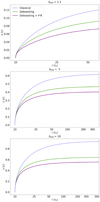Fig. 1. Representation of the evolution of the wind velocity (in units of c) as a function of radial distance (in units of rS and in log scale) and for super-Eddington luminosities. The velocity evolution is plotted whilst neglecting special relativistic effects (in blue), or neglecting the P–R effect (in green), or considering it (in purple). The wind is assumed to be launched from r0 = 10rS with zero initial radial velocity.

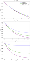Fig. 2. Representation of the evolution of the wind velocity (in units of c) as a function of radial distance (in units of rS and in log scale) and for sub-Eddington luminosities. The velocity evolution is plotted whilst neglecting special relativistic effects (in blue), or neglecting the P–R effect (in green), or considering it (in purple). The wind is assumed to be launched from r0 = 10rS with initial velocity equal to the escape velocity.

For the super-Eddington luminosities, the velocity of the wind taking into account the P–R effect is between 14% and 24% lower than that when neglecting the effect after a dimensionless time interval Δt_• = 10³ (which, assuming M_BH = 10⁸ M_⊙, would be equal to a time interval Δt ≃ 10⁶s ≃ 12 days). The difference is between 41% and 43% if we also neglect the deboosting factor. In the case of the sub-Eddington luminosities, the velocity of the wind when taking into account the P–R effect is between 10% and 12% lower than that when neglecting the effect and is between 22% and 26% lower than the case where we neglect the deboosting factor in addition to neglecting the P–R effect.

The importance of the effect clearly varies according to the velocity of the wind. We now study the force exerted by the radiation pressure as a function of the velocity of the wind. Because of the effect described in Eq. (1), the radiation that reaches the wind is maximum when the wind moves with velocity v = 0. Therefore, the maximum value of the force exerted by the radiation pressure is reached for v = 0 and we normalize this value to 1 (for the sake of simplicity, we assume that the radial coordinate is fixed). With this normalisation, the force caused by radiation whilst neglecting or considering the P-R effect is, respectively (see Fig. 3)

$$\begin{array}{cc}& {\mathit{F}}_{\mathrm{rad}}=(1-\beta )\mathit{n},\hfill \end{array}$$(36)

$$\begin{array}{cc}& {\mathit{F}}_{\mathrm{rad}}^{\mathrm{PR}}=[1-\beta -\frac{\beta (1-\beta )}{1+\beta }]\mathit{n}.\hfill \end{array}$$(37)

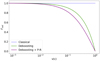Fig. 3. Representation of the force exerted by the radiation as a function of the velocity of the wind, whilst neglecting special relativistic effects (in blue), or neglecting the P–R effect (in green), or considering it (in purple).

Subtracting Eq. (36) from Eq. (37), we obtain a factor −Ω_PR, which quantifies the importance of the P–R effect as a function of the velocity of the wind, applying the same normalization as that used for describing the force exerted by the radiation (the minus sign indicates that the P–R effect slows the atom down). We define the Poynting–Robertson factor as

$$\begin{array}{c}\hfill {\mathrm{\Omega }}_{\mathrm{PR}}=\frac{\beta (1-\beta )}{1+\beta }.\end{array}$$(38)

Using Eq. (38) in Eq. (34), we obtain

$$\begin{array}{c}\hfill \frac{{\mathrm{d}}^2{r}_{\bullet }}{\mathrm{d}{t}_{\bullet }^2}+\frac{1}{2{(r_{\bullet }-1)}^2}+\frac{{\lambda }_{\mathrm{Edd}}}{2r_{\bullet }^2}(-1+\beta +{\mathrm{\Omega }}_{\mathrm{PR}})=0.\end{array}$$(39)

As seen in Fig. 4, the factor Ω_PR is = 0 when v = 0. Indeed, in this situation, the Lorentz transformation, which is responsible for the anisotropy of the emitted radiation, is absent. However, the effect is also negligible in the limit in which the wind moves with the same velocity as light. Indeed, because of relativistic corrections, the wind does not perceive any radiation and so there is no re-emission. This is consistent with the deboosting factor described in Eq. (1). Furthermore, we notice that the factor Ω_PR assumes its maximum value of ∼17.2% (and so the P–R effect is maximum) when the velocity is ∼0.41 c.

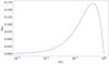Fig. 4. Representation of the Poynting–Robertson factor (defined in Eq. (38)) as a function of the velocity of the wind (expressed in units of c).

4. Discussion and conclusions

In this paper, we present our study of the Poynting–Robertson effect and its application on the dynamics of UFOs driven by accreting black holes. We present a special relativistic derivation of the effect and we derived Eqs. (25)–(27) to use in order to easily implement the effect in future, more complex simulation works (Sect. 2). Here, we implement it in a simple case in which we assume that the wind can be described with a toy model in which the wind particle moves radially and the motion is dominated by the gravitational force and the force exerted by the radiation pressure. Furthermore, we present a model based on the retarded potentials in order to evaluate the radiation emitted by a charged particle of the ionized wind and we show that this term is negligible with respect to the radiation from the illuminating source (see Appendix A). It is essential to take into account relativistic corrections in order to build a proper modeling of UFOs and high-velocity astrophysical flows in general (see Luminari et al. 2020, 2021). In this work, we show that the Poynting–Robertson effect also plays an important role in the description of the dynamics of the wind, especially for mildly to highly relativistic velocities (see Fig. 4). Neglecting the P–R effect, the velocity of the wind would be largely overestimated. This effect contributes to demonstrating the importance of special relativistic corrections for a precise description of the properties of the wind, a precision that will become even more important with the next generation of X-ray telescopes, such as XRISM and Athena. In future works, we plan to couple the P–R effect with magneto-hydrodynamic acceleration in order to develop more accurate simulations that can properly describe the dynamics of the wind and predict the terminal velocity that can be reached. Our model could also be improved by taking into account different sizes and geometries for the source of radiation. Indeed, while the X-ray corona could be assumed point-like (as in this work), the distribution of the accretion disk could modify the radiation term in the optical–UV band (Nardini et al. 2016). For nonradial photon flux, the velocity reduction factor would depend on the angular coordinates and the strongest reduction would be along the direction of motion.

Acknowledgments

This article was part of the Bachelor Thesis in Physics at the Tor Vergata University of Rome by MM. AL acknowledges support from the HORIZON-2020 grant “Integrated Activities for the High Energy Astrophysics Domain” (AHEAD-2020), G.A. 871158.

References

Appendix A: Radiation generated by a moving charged particle

In this section, we derive the expression for the radiation emitted by a moving charged particle. Here, we compute the first three terms of the expression in order to prove that the terms successive to the electric dipole are suppressed by increasing orders of c. Then, we show that the dipole term is negligible when compared to the contribution of radiation from the illuminating source. To do this calculation, we use the retarded vector potential (see Jackson (1962) for further details):

$$\begin{array}{c}\hfill \mathit{A}(t,\mathit{x})={\displaystyle \int }\frac{d^3{x}^{\prime }}{c}\frac{\mathit{J}(t^{\prime }=t-\frac{|\mathit{x}-{\mathit{x}}^{\prime }|}{c},{\mathit{x}}^{\prime })}{|\mathit{x}-{\mathit{x}}^{\prime }|},\end{array}$$(A.1)

where x is the position in which we are evaluating the potential and x′ is the position of the radiation source. Assuming |x|≫|x′| we obtain

$$\begin{array}{cc}\hfill \mathit{A}(t,\mathit{x})\simeq & \frac{1}{\mathit{cr}}{\displaystyle \int }{d}^3{x}^{\prime }\mathit{J}(t^{\prime }=t-\frac{r}{c},{\mathit{x}}^{\prime })+\hfill \\ \hfill +& \frac{1}{\mathit{cr}}{\displaystyle \int }{d}^3{x}^{\prime }\frac{\mathit{n}·{\mathit{x}}^{\prime }}{c}\frac{\partial }{\partial t}\mathit{J}(t,{\mathit{x}}^{\prime }){|}_{t^{\prime }=t-\frac{r}{c}},\hfill \end{array}$$(A.2)

where r = |x| and $\mathit{n}=\frac{\mathit{x}}{r}$. We denote the first term of Eq. (A.2) A₁ and the second term A₂. As

$$\begin{array}{c}\hfill \mathit{J}({\mathit{x}}^{\prime },t)={\displaystyle \sum _a{q}_a{\mathit{v}}_a\delta ({\mathit{x}}^{\prime }-{\mathit{x}}_a(t)),}\end{array}$$(A.3)

where the sum does not appear if we are considering a single particle, we obtain

$$\begin{array}{c}\hfill {\mathit{A}}_1=\frac{[\mathit{p}]}{\mathit{rc}},\end{array}$$(A.4)

where we use Newton’s notation for time derivatives and the symbol [ ] to indicate that the argument inside the parentheses must be evaluated at time $t^{\prime }=t-\frac{r}{c}$. For A₂, using the identity ${\mathit{v}}_a(\mathit{n}·{\mathit{x}}_a)=\frac{1}{2}({\mathit{x}}_a\times {\mathit{v}}_a)\times \mathit{n}+\frac{1}{2}\frac{d}{\mathit{dt}}[{\mathit{x}}_a(\mathit{n}·{\mathit{x}}_a)]$, we obtain

$$\begin{array}{cc}\hfill {\mathit{A}}_2=& \frac{1}{2c{r}^2}\{\frac{d^2}{d{t}^2}{\displaystyle \sum _a}{q}_a\left[{\mathit{x}}_a(\mathit{n}·{\mathit{x}}_a)\right]+\hfill \\ \hfill +& \frac{d}{\mathit{dt}}{\displaystyle \sum _a{q}_a({\mathit{x}}_a\times {\mathit{v}}_a)\times \mathit{n}{\}}_{t^{\prime }=t-\frac{r}{c}}.}\hfill \end{array}$$(A.5)

The first term of Eq. (A.5) can be connected to the magnetic dipole $\mathit{\mu }=\sum _a\frac{q_a}{2m_{a}c}({\mathit{x}}_a\times m_a{\mathit{v}}_a)$ and the second term to the electric quadrupole moment ${\mathbb{Q}}_{ij}=\sum _a{q}_a(3x_{\text{i}}^a{x}_j^a-{\delta }_{ij}|x_a^2{|}^2)$, obtaining

$$\begin{array}{c}\hfill {\mathit{A}}_2=\frac{[\mathit{Q}]}{6c^{2}r}+\frac{[\mathit{\mu }]\times \mathit{n}}{\mathit{cr}}.\end{array}$$(A.6)

From the conservation of energy equation $\frac{\partial \omega }{\partial t}=-\mathbf{\nabla }·\mathit{S}$ (where ω is the energy density and $\mathit{S}=\frac{{c|\mathit{B}|}^2}{4\pi }\mathit{n}$ is the Poynting vector) it follows that

$$\begin{array}{c}\hfill -\frac{d\mathcal{E}}{\mathit{dt}}=P_{\mathit{emitted}}={\displaystyle \int }d\mathrm{\Omega }{r}^2\frac{c|{\mathit{B}}^2|}{4\pi },\end{array}$$(A.7)

and so

$$\begin{array}{c}\hfill \frac{d{P}_{\mathit{emitted}}}{d\mathrm{\Omega }}=\frac{{c|\mathit{B}|}^2}{4\pi }{r}^2.\end{array}$$(A.8)

As we are in the hypothesis |x|≫|x′| and as we can put the scalar potential equal to 0 because of radiation gauge, it follows that $\mathit{E}=-\frac{1}{c}\frac{\partial \mathit{A}}{\partial t}$ and $\mathit{B}=\mathbf{\nabla }\times \mathit{A}=\frac{1}{c}\frac{\partial \mathit{A}}{\partial t}\times \mathit{n}$. Therefore, we finally obtain the expression

$$\begin{array}{cc}\hfill \frac{\mathit{dP}}{d\mathrm{\Omega }}& =\frac{1}{4\pi c^3}{\{|\mathit{p}\times \mathit{n}|}^2+\frac{1}{36c^2}|\stackrel{⃛}{\mathit{Q}}{\times \mathit{n}|}^2+{|(\mathit{\mu }\times \mathit{n})\times \mathit{n}|}^2+\hfill \\ \hfill & +\frac{1}{3c}(\mathit{p}\times \mathit{n})·(\stackrel{⃛}{\mathit{Q}}\times \mathit{n})+2(\mathit{p}·[(\mathit{\mu }\times \mathit{n})\times \mathit{n}]+\hfill \\ \hfill & +\frac{1}{3c}(\stackrel{⃛}{\mathit{Q}}\times \mathit{n})·[(\mathit{\mu }\times \mathit{n})\times \mathit{n}]\}.\hfill \end{array}$$(A.9)

Because of symmetry reasons, it follows that $\int \frac{d\mathrm{\Omega }}{4\pi }=1$, $\frac{d\mathrm{\Omega }}{4\pi }{n}^i=0$, $\int \frac{d\mathrm{\Omega }}{4\pi }{n}^i{n}^j=\frac{1}{3}{\delta }^{\mathit{ij}}$, $\int \frac{d\mathrm{\Omega }}{4\pi }{n}^i{n}^j{n}^k=0$ and $\int \frac{d\mathrm{\Omega }}{4\pi }{n}^i{n}^j{n}^k{n}^l=\frac{1}{15}({\delta }^{\mathit{ij}}{\delta }^{\mathit{kl}}+{\delta }^{\mathit{ik}}{\delta }^{\mathit{jl}}+{\delta }^{\mathit{il}}{\delta }^{\mathit{jk}})$ and so, integrating the last three terms of Eq. (A.9), we obtain 0. For the first three terms, we instead obtain

$$\begin{array}{cc}\hfill P_{\mathit{emitted}}& =\frac{2}{3c^3}{[\mathit{p}]}^2+\frac{2}{3c^3}{[\mathit{\mu }]}^2\hfill \\ \hfill & +\frac{1}{180c^5}[Tr(\stackrel{⃛}{\mathbb{Q}}\stackrel{⃛}{\mathbb{Q}})-\frac{1}{3}{(Tr\stackrel{⃛}{\mathbb{Q}})}^2]+\text{futher terms}.\hfill \end{array}$$(A.10)

The terms given by the magnetic dipole moment μ and the electric quadrupole tensor ℚ give a contribution suppressed by higher orders of c compared to that of the electric dipole moment p (there is a factor $\frac{1}{c}$ in the definition of μ). We therefore focus on the term given by the electric dipole moment for which, from Eq. (A.9), it follows that

$$\begin{array}{c}\hfill \frac{d{P}_{\mathit{emitted}}}{d\mathrm{\Omega }}=\frac{1}{4\pi c^3}{|\mathit{p}|}^2(1-co{s}^2\theta ).\end{array}$$(A.11)

It is evident that the power emitted is the same for angles θ and θ + π and so the particle is not subjected to a force caused by the emission of radiation in its reference frame. The dipole term is suppressed by orders of c³, while the radiation from the accreting black hole (which we assumed to be completely absorbed and re-emitted by the wind) is generally much greater, because we consider luminosities near the Eddington limit. In the main text of this work, we therefore neglect the dipole term. However, exploiting the symmetry of the term, it could be easily taken into account, repeating the same derivation presented in Sect. 2.

All Figures

Fig. 1. Representation of the evolution of the wind velocity (in units of c) as a function of radial distance (in units of rS and in log scale) and for super-Eddington luminosities. The velocity evolution is plotted whilst neglecting special relativistic effects (in blue), or neglecting the P–R effect (in green), or considering it (in purple). The wind is assumed to be launched from r0 = 10rS with zero initial radial velocity.

In the text

Fig. 2. Representation of the evolution of the wind velocity (in units of c) as a function of radial distance (in units of rS and in log scale) and for sub-Eddington luminosities. The velocity evolution is plotted whilst neglecting special relativistic effects (in blue), or neglecting the P–R effect (in green), or considering it (in purple). The wind is assumed to be launched from r0 = 10rS with initial velocity equal to the escape velocity.

In the text

	Fig. 3. Representation of the force exerted by the radiation as a function of the velocity of the wind, whilst neglecting special relativistic effects (in blue), or neglecting the P–R effect (in green), or considering it (in purple).
In the text

	Fig. 4. Representation of the Poynting–Robertson factor (defined in Eq. (38)) as a function of the velocity of the wind (expressed in units of c).
In the text

References

- Cappi, M., Tombesi, F., Bianchi, S., et al. 2009, A&A, 504, 401 [NASA ADS] [CrossRef] [EDP Sciences] [Google Scholar]
- Chartas, G., Cappi, M., Vignali, C., et al. 2021, ApJ, 920, 24 [NASA ADS] [CrossRef] [Google Scholar]
- Chattopadhyay, I. 2005, MNRAS, 356, 145 [NASA ADS] [CrossRef] [Google Scholar]
- Fiore, F., Feruglio, C., Shankar, F., et al. 2017, A&A, 601, A143 [NASA ADS] [CrossRef] [EDP Sciences] [Google Scholar]
- Fukue, J. 1996, PASJ, 48, 631 [NASA ADS] [CrossRef] [Google Scholar]
- Fukumura, K., Kazanas, D., Contopoulos, I., et al. 2010, ApJ, 715, 636 [NASA ADS] [CrossRef] [Google Scholar]
- Fukumura, K., Tombesi, F., Kazanas, D., et al. 2015, ApJ, 805, 17 [NASA ADS] [CrossRef] [Google Scholar]
- Gofford, J., Reeves, J. N., Tombesi, F., et al. 2013, MNRAS, 430, 60 [Google Scholar]
- Hsieh, S.-H., & Spiegel, E. A. 1976, ApJ, 207, 244 [NASA ADS] [CrossRef] [Google Scholar]
- Jackson, J. D. 1962, Classical Electrodynamics (New York: John Wiley& Sons, Inc.) [Google Scholar]
- Klacka, J. 1992, Earth Moon Planets, 59, 41 [NASA ADS] [CrossRef] [Google Scholar]
- Kormendy, J., & Ho, L. C. 2013, ARA&A, 51, 511 [Google Scholar]
- Landau, L. D., & Lifshitz, E. M. 1951, The Classical Theory of Fields, 2 [Google Scholar]
- Luminari, A., Tombesi, F., Piconcelli, E., et al. 2020, A&A, 633, A55 [NASA ADS] [CrossRef] [EDP Sciences] [Google Scholar]
- Luminari, A., Nicastro, F., Elvis, M., et al. 2021, A&A, 646, A111 [NASA ADS] [CrossRef] [EDP Sciences] [Google Scholar]
- Mizumoto, M., Nomura, M., Done, C., et al. 2021, MNRAS, 503, 1442 [CrossRef] [Google Scholar]
- Nardini, E., Porquet, D., Reeves, J. N., et al. 2016, ApJ, 832, 45 [NASA ADS] [CrossRef] [Google Scholar]
- Nomura, M., Ohsuga, K., Takahashi, H. R., et al. 2016, PASJ, 68, 16 [NASA ADS] [CrossRef] [Google Scholar]
- Paczyńsky, B., & Wiita, P. J. 1980, A&A, 88, 23 [NASA ADS] [Google Scholar]
- Pounds, K. A., Reeves, J. N., King, A. R., et al. 2003, MNRAS, 345, 705 [Google Scholar]
- Poynting, J. H. 1903, MNRAS, 64, 1 [Google Scholar]
- Poynting, J. H. 1904, A, 202, 525 . Phil. Trans. Royal Soc. London Ser. [Google Scholar]
- Quera-Bofarull, A., Done, C., Lacey, C. G., et al. 2021, ArXiv e-prints [arXiv:2111.02742] [Google Scholar]
- Raychaudhuri, S., Vyas, M. K., & Chattopadhyay, I. 2021, MNRAS, 501, 4850 [NASA ADS] [CrossRef] [Google Scholar]
- Robertson, H. P. 1937, MNRAS, 97, 423 [NASA ADS] [Google Scholar]
- Rybicki, G. B., & Lightman, A. P. 1986, Radiative Processes in Astrophysics (New York: Wiley-VCH), 400 [Google Scholar]
- Sim, S. A., Proga, D., Kurosawa, R., et al. 2012, MNRAS, 426, 2859 [NASA ADS] [CrossRef] [Google Scholar]
- Takahashi, H. R., & Ohsuga, K. 2015, PASJ, 67, 60 [NASA ADS] [CrossRef] [Google Scholar]
- Tombesi, F., Cappi, M., Reeves, J. N., et al. 2010, A&A, 521, A57 [NASA ADS] [CrossRef] [EDP Sciences] [Google Scholar]
- Yang, X.-H. 2021, ApJ, 922, 262 [NASA ADS] [CrossRef] [Google Scholar]