| Issue |
A&A
Volume 642, October 2020
|
|
|---|---|---|
| Article Number | L9 | |
| Number of page(s) | 4 | |
| Section | Letters to the Editor | |
| DOI | https://doi.org/10.1051/0004-6361/202039246 | |
| Published online | 06 October 2020 | |
Letter to the Editor
The Djorgovski–Gurzadyan dark energy integral equation and the Hubble diagram
1
Center for Cosmology and Astrophysics, Alikhanian National Laboratory, Yerevan, Armenia
e-mail: harut@mail.yerphi.am
2
Yerevan State University, Yerevan, Armenia
Received:
24
August
2020
Accepted:
15
September
2020
We consider the observational aspects of the value of dark energy density from quantum vacuum fluctuations based initially on the Gurzadyan–Xue model. We reduce the Djorgovski–Gurzadyan integral equation to a differential equation for the co-moving horizon and then, by means of the obtained explicit form for the luminosity distance, we construct the Hubble diagram for two classes of observational samples. For supernova and gamma-ray burst data we show that this approach provides viable predictions for distances up to z ≃ 9, quantitatively at least as good as those provided by the Λ cold dark matter model. The Hubble parameter dependence H(z) of the two models also reveals mutual crossing at z = 0.4018, the interpretation of which is less evident.
Key words: cosmological parameters / cosmology: observations / dark energy / cosmology: theory
© ESO 2020
1. Introduction
In his pioneering work Zeldovich (1967, 1968) assigned the cosmological constant Λ, if non-zero, as a contribution of quantum vacuum fluctuations with the ϵ = −p equation of state (EOS; energy ϵ and pressure p). After the discovery of the accelerated expansion of the Universe a number of models and approaches were proposed (see Copeland et al. 2006), typically involving either theoretical or phenomenological input parameters.
Among the proposed approaches, Gurzadyan–Xue (GX) models do not have any free or empirical parameters, and they predict a value of Λ fitting its observed value. This class of models (see Khachatryan et al. 2007; Khachatryan 2007; Vereshchagin 2006; Vereshchagin & Yegorian 2006a,b, 2008) also covers those parameters with a variation of fundamental constants, and has been tested regarding the Hubble diagram using the supernova (SN) and gamma-ray burst (GRB) observational data Mosquera Cuesta et al. (2008).
Djorgovski & Gurzadyan (2007, hereafter DG) did an in-depth refinement while comparing these models to the observational data; in other words, they reconsidered the concept of one of the key parameters in the GX formula, the maximum distance Lmax assigned to the quantum fluctuations. By setting this distance to co-moving horizon, they got a parameter-free integral equation, which they solved iteratively. In this paper we switch the DG equation to a differential one, avoiding the arising of an integration constant, and obtain a value of dark energy density again without any other assumptions except on the empirical values of the matter density and the curvature of the Universe; we also derive the Hubble diagram for available SN and GRB data samples.
The paper is organized as follows. In the first part we derive the main formulae and get a numerical solution for parameter y(z). Then we construct Hubble diagrams for SN and GRB samples and compare Hubble parameter graphs for the Λ cold dark matter (ΛCDM) model and the GX–DG model. While the observational data seem to support the EOS parameter w(z) ≈ − 1 for dark energy (Astier et al. 2006; Riess et al. 2004, 2007), we derive an equation for w(z) and see that it slightly varies with redshift. We also consider some further cosmological insights on the considered dark energy scalings.
2. Dark energy versus luminosity distance
In their original work Gurzadyan & Xue (2002, 2003) proposed considering, in the dark energy only, the contribution of l = 0 spherical modes of vacuum fluctuations. As was well known, accounting for all vacuum fluctuations leads to about 10123 quantitative discrepancies of the theoretical density with the empirical dark energy value. Thus, they derived a simple equation for dark energy density,
where DH = c/H0 is the Hubble horizon scale, i.e., the distance that light would travel during Hubble time 1/H0.
The key issue with Eq. (1) is what to choose for the maximum distance Lmax associated with the fluctuations. In some papers (Vereshchagin 2006; Vereshchagin & Yegorian 2006a,b, 2008; Khachatryan et al. 2007; Khachatryan 2007) the scale factor is used as a maximum distance and that assumption gave ΩΛ ≈ 3.29 for dark energy density, while the observed value is ≈0.7).
Djorgovski & Gurzadyan (2007) suggested another solution for the choice of the maximum distance Lmax, namely using the distance to the horizon measured in co-moving units
where D∞ and h(z) = H(z)/H0 are the distance to the horizon and a dimensionless Hubble parameter, respectively. As a result they obtained only a 20% difference between the theoretical and observed values of the dark energy density. This integral equation can be rewritten in the form of differential equation for y(z) parameter
This equation assumes that in the early Universe z → ∞ the Hubble parameter H(z)→∞.
The initial condition for y′ follows from the Friedmann equations and can be rewritten as  . Here we consider only flat k = 0, Ωk = 0 case, but the equation is true for any k.
Equation (3) cannot be solved analytically and the numerical solution is depicted in Fig. 1.
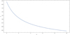 |
Fig. 1. Numerical solution of Eq. (3) for redshift z up to 10. Model parameters are set to Ωm = 0.315, Ωr = 1.08622 × 10⁻⁵. |
To construct the Hubble diagram the luminosity distance and the distance moduli are needed. They can be expressed by y(z) in a simple form
3. Hubble diagram
In this section we construct the Hubble diagram for the Union2.1 sample of SN Ia (Amanullah et al. 2010; Suzuki et al. 2012). We used a standard parameter set for the numerical solution of y(z) (see Fig. 1). It shows that the standard model with a cosmological constant predicts values that are a bit higher for distance moduli of SNs (Fig. 2). The χ2 values for ΛCDM model are somewhat smaller than for the DG-GX model, χ2 = 1.1 and χ2 = 1.29, respectively.
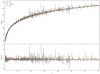 |
Fig. 2. Hubble diagram for 580 SNs of the Union2.1 SN Ia sample (Amanullah et al. 2010; Suzuki et al. 2012). The red solid line represents the GX–DG cosmological model and the green solid line the ΛCDM model. The Hubble constant value is taken as H0 = 70 km s−1 Mpc−1. |
We also fit the models with GRB data from Demianski et al. (2017), which were calibrated independently using Amati relation and can be used with any dark energy model. The Amati relation (Amati 2006) refers to an empirical relation between isotropic equivalent radiated energy Eiso and the observed photon energy of the peak spectral fluxEp, i:
![$$ \begin{aligned} \log \left(\frac{E_{\rm iso}}{1\,\mathrm{erg}}\right)=b+a\log \left[\frac{E_{p,i}}{300\,\mathrm{KeV}}\right]\cdot \end{aligned} $$](/articles/aa/full_html/2020/10/aa39246-20/aa39246-20-eq6.gif)
The Amati relation is known to be not applicable for any GRBs with measured parameter pairs Eiso, Ep, i (see Qin & Chen 2013; Lin et al. 2015); moreover, the regression parameters a, b slightly differ when obtained by different authors. Although the Amati relation was nevertheless concluded to be the preferable to other empirical relations for GRBs while constructing the Hubble diagram (Wang et al. 2020), more detailed work is indeed needed in the future in the comparative analysis of various empirical relations and their possibly combined applications.
For GRBs we see that the GX–DG model fits better: for the ΛCDM model we have χ2 = 1.41 and for the GX–DG model χ2 = 1.21. This can be seen even in Fig. 3, where the GRB distance moduli values are smaller and therefore the GX–DG model fits better. To trace the statistical properties of the GRB data we fitted and then calculated χ2, for example for the GRB data from Liu & Wei (2015) as well; we obtained lower values for χ2 (0.4271, 0.4319) for the GX–DG and ΛCDM models, respectively.
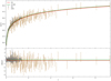 |
Fig. 3. Hubble diagram for 580 SNs of the Union2.1 SN Ia sample and 162 calibrated GRBs from Demianski et al. (2017). The red line represents the GX–DG cosmological model and the green line the ΛCDM model. |
Then we plot in Fig. 4 the Hubble parameter dependence on the redshift for different values H0 = 67.4, 73.24 km s−1 Mpc−1 for the ΛCDM and the GX–DG model; we chose the Hubble parameter because the Planck satellite data on the Cosmic Microwave Background (CMB) (Planck Collaboration VI 2020) provide the Hubble constant value H0 = 67.4 ± 0.5 km s−1 Mpc−1, while the Milky Way Cepheid survey (Riess et al. 2018, 2019) suggests H0 = 73.24 ± 1.62 km s−1 Mpc−1. We note that the graph with the GX–DG model for the Hubble constant value H0 = 67.4 km s−1 Mpc−1 crosses at around z = 0.4018 the graph of the ΛCDM model with Hubble constant value H0 = 73.24 km s−1 Mpc−1; i.e., at redshifts lower than z = 0.4018 the Hubble parameter for GX–DG model approximate ΛCDM model’s graph with H0 = 67.4 km s−1 Mpc−1 and at higher redshifts tending to that of H0 = 73.24 km s−1 Mpc−1.
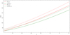 |
Fig. 4. Hubble parameter H(z) dependance on the redshift z. The red lines represent GX–DG cosmological model and the green lines refer to the ΛCDM model (dashed H0 = 73.24 km s−1 Mpc−1, dotted H0 = 67.4 km s−1 Mpc−1. |
The interpretation of this result, and whether it is related to the Hubble parameter issues in Verde et al. (2019), is not clear. We can predict, to be confirmed or ruled out at future observations, that at z = 0.4018 either the Hubble parameter or the parameter w, or some other related parameter undergoes a change in properties.
4. Equation of state parameter
In the standard ΛCDM model dark energy is adopted as the cosmological constant. Therefore, it is important to have an equation for the EOS parameter w(z) dependence on redshift for the GX–DG model; for ΛCDM w(z)≈ − 1. From Eq. (3) we can easily derive a formula for the EOS parameter
In Fig. 5 we can see the dependance of the EOS parameter on the redshift. It is negative in a wide range of redshifts, but at around z ≈ 6 it turns to zero.
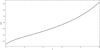 |
Fig. 5. Effective EOS parameter w(z) as a function of redshift z. |
5. Information evolution
In this section we link the GX–DG model to the “information” description of the cosmological evolution (Gurzadyan & Stepanian 2019). Thus, the vacuum matter density is
where Lpl is the Planck length and Lmax is the upper bound of the vacuum modes, which is considered the cosmological horizon in co-moving coordinates (Djorgovski & Gurzadyan 2007).
Within the framework of the information evolution (IE), it is assumed that the evolution of the Universe can be described according to the increase of a discretized quantity, the information. This concept is obtained based on the notion of Bekenstein Bound (Bekenstein 1981), which introduces an upper bound of information

where R and E are the characteristic radius and energy of a system under the consideration. Thus, the evolution of the Universe (T) is discretized as follows:
Accordingly, at each stage (j) of IE, the Universe is denoted by the characteristic mass Mj and radius Rj
where  is the Hubble horizon at that stage. On the one hand, IBB is inversely proportional to the total density of the Universe and Eq. (9) can be written as
On the other hand, the evolution of the Universe can be described based on the area of the cosmological horizon at each stage Aj, i.e.,

so that the information content of Universe increases until the area of the Hubble horizon reaches  , the de Sitter cosmological horizon. Consequently, at this stage the density becomes
  . Thus, in the context of IE

Then, the “maximum number of relevant radial modes” in the GX model is defined as
Comparing these relations with the notion of area in IE leads us to the following degrees of freedom
Thus, by comparing Eq. (7) with the notions of “area of cosmological horizon” and “matter density” we can conclude that the results of GX–DG and IE models, although assuming entirely different approaches, are similar. It should be noted that this similarity exists only if ρ in Eq. (7) corresponds to the total density of the Universe (according to Eq. (11)).
Obviously, the two approaches deal with certain global scaling parameters and they should be reduced to standard Friedmann–Lemaitre–Robertson–Walker universe with the continuous geometrical structure.
6. Conclusions
We reduced the Djorgovski & Gurzadyan (2007) integral equation to a differential equation to describe dark energy with observable parameters. Solving that differential equation we obtained the exact value of dark energy density. This allowed us to construct the Hubble diagram for SN and GRB samples and to show that the model estimates the observed distances up to z ≃ 9 at least as well as the standard ΛCDM model with a cosmological constant. The dark energy EOS parameter predicts a slight variation with redshift which is still not observable, however.
The behavior of the GX–DG model and comparison with observational data shows that if there are no unknown experimental systematics (Niedermann & Sloth 2008; Efstathiou 2014, 2020), the GX–DG model can be adopted along with the standard ΛCDM model. The revealed feature of the diagrams, namely, the crossing of the curves of both models at z = 0.4018 is not obvious for direct interpretation, suggesting possible different behaviors of parameters at redshifts z < 0.4018 and z > 0.4018, as a test to be solved by means of future observations. Finally, regarding the DG integral equation we note that the first-order differential equation for dark energy density Eq. (3) has one integration invariant that can be related to the invariants of the general equations of GX models (Khachatryan 2007).
Acknowledgments
We are thankful to the referee for very useful comments and suggestions that helped to improve the paper.
References
- Amanullah, R., Lidman, C., Rubin, D., et al. 2010, ApJ, 716, 713 [Google Scholar]
- Amati, L. 2006, MNRAS, 372, 233 [NASA ADS] [CrossRef] [Google Scholar]
- Astier, P., Guy, J., Regnault, N., et al. 2006, A&A, 447, 31 [NASA ADS] [CrossRef] [EDP Sciences] [Google Scholar]
- Bekenstein, J. D. 1981, Phys. Rev. D, 23, 287 [NASA ADS] [CrossRef] [MathSciNet] [Google Scholar]
- Copeland, E. J., Sami, M., & Tsujikawa, S. 2006, Int. J. Mod. Phys. D, 15, 1753 [NASA ADS] [CrossRef] [MathSciNet] [Google Scholar]
- Demianski, M., Piedipalumbo, E., Sawant, D., & Amati, L. 2017, A&A, 598, A112 [NASA ADS] [CrossRef] [EDP Sciences] [Google Scholar]
- Djorgovski, S. G., & Gurzadyan, V. G. 2007, Nucl. Phys. B, 173, 6 [CrossRef] [Google Scholar]
- Efstathiou, G. 2014, MNRAS, 440, 1138 [NASA ADS] [CrossRef] [Google Scholar]
- Efstathiou, G. 2020, ArXiv e-prints [arXiv:2007.10716] [Google Scholar]
- Gurzadyan, V. G., & Stepanian, A. 2019, Eur. Phys. J. Plus, 134, 98 [CrossRef] [Google Scholar]
- Gurzadyan, V. G., & Xue, S.-S. 2002, From Integrable Models to Gauge Theories (World Scientific), 177 [CrossRef] [Google Scholar]
- Gurzadyan, V. G., & Xue, S.-S. 2003, Mod. Phys. Lett. A, 18, 561 [NASA ADS] [CrossRef] [Google Scholar]
- Huterer, D., & Shafer, D. L. 2018, Rep. Prog. Phys., 81, 016901 [NASA ADS] [CrossRef] [Google Scholar]
- Khachatryan, H. G. 2007, Mod. Phys. Lett. A, 22, 333 [NASA ADS] [CrossRef] [Google Scholar]
- Khachatryan, H. G., Vereshchagin, G. V., & Yegorian, G. 2007, Il Nuovo Cimento B, 122, 197 [NASA ADS] [Google Scholar]
- Lin, H.-N., Li, X., Wang, S., & Chang, Z. 2015, MNRAS, 453, 128 [NASA ADS] [CrossRef] [Google Scholar]
- Liu, J., & Wei, H. 2015, Gen. Rel. Grav., 47, 141 [NASA ADS] [CrossRef] [Google Scholar]
- Mosquera Cuesta, H. J., Turcati, R., Furlanetto, C., et al. 2008, A&A, 487, 47 [NASA ADS] [CrossRef] [EDP Sciences] [Google Scholar]
- Niedermann, F., & Sloth, M. S. 2019, ArXiv e-prints [arXiv:1910.10739] [Google Scholar]
- Peebles, P. J. E. 1993, Principles of Physical Cosmology (Press: Princeton Univ) [Google Scholar]
- Planck Collaboration VI. 2020, A&A, 641, A6 [NASA ADS] [CrossRef] [EDP Sciences] [Google Scholar]
- Qin, Y.-P., & Chen, Z.-F. 2013, MNRAS, 430, 163 [CrossRef] [Google Scholar]
- Riess, A., Strolger, L. G., Tonry, J., et al. 2004, ApJ, 607, 665 [NASA ADS] [CrossRef] [Google Scholar]
- Riess, A., Strolger, L. G., Casertano, S., et al. 2007, ApJ, 659, 98 [NASA ADS] [CrossRef] [Google Scholar]
- Riess, A., Casertano, S., Yuan, W., et al. 2018, ApJ, 861, 121 [Google Scholar]
- Riess, A. G., Casertano, S., Yuan, W., et al. 2019, ApJ, 876, 85 [NASA ADS] [CrossRef] [Google Scholar]
- Suzuki, N., Rubin, D., Lidman, C., et al. 2012, ApJ, 746, 1 [NASA ADS] [CrossRef] [Google Scholar]
- Verde, L., Treu, T., & Riess, A. G. 2019, Nat. Astron., 3, 891 [NASA ADS] [CrossRef] [Google Scholar]
- Vereshchagin, G. V. 2006, Mod. Phys. Lett. A, 21, 729 [NASA ADS] [CrossRef] [Google Scholar]
- Vereshchagin, G. V., & Yegorian, G. 2006a, Phys. Lett. B, 636, 150 [NASA ADS] [CrossRef] [Google Scholar]
- Vereshchagin, G. V., & Yegorian, G. 2006b, Class. Quantum Grav., 23, 5049 [NASA ADS] [CrossRef] [Google Scholar]
- Vereshchagin, G. V., & Yegorian, G. 2008, Int. J. Mod. Phys. D, 17, 203 [NASA ADS] [CrossRef] [Google Scholar]
- Wang, F., Zou, Y. C., Liu, F., et al. 2020, ApJ, 893, 77 [CrossRef] [Google Scholar]
- Zeldovich, Y. B. 1967, JETP Lett., 6, 883 [Google Scholar]
- Zeldovich, Y. B. 1968, Sov. Phys. Uspekhi, 95, 209 [Google Scholar]
All Figures
|
Fig. 1. Numerical solution of Eq. (3) for redshift z up to 10. Model parameters are set to Ωm = 0.315, Ωr = 1.08622 × 10⁻⁵. |
| In the text | |
|
Fig. 2. Hubble diagram for 580 SNs of the Union2.1 SN Ia sample (Amanullah et al. 2010; Suzuki et al. 2012). The red solid line represents the GX–DG cosmological model and the green solid line the ΛCDM model. The Hubble constant value is taken as H0 = 70 km s−1 Mpc−1. |
| In the text | |
|
Fig. 3. Hubble diagram for 580 SNs of the Union2.1 SN Ia sample and 162 calibrated GRBs from Demianski et al. (2017). The red line represents the GX–DG cosmological model and the green line the ΛCDM model. |
| In the text | |
|
Fig. 4. Hubble parameter H(z) dependance on the redshift z. The red lines represent GX–DG cosmological model and the green lines refer to the ΛCDM model (dashed H0 = 73.24 km s−1 Mpc−1, dotted H0 = 67.4 km s−1 Mpc−1. |
| In the text | |
|
Fig. 5. Effective EOS parameter w(z) as a function of redshift z. |
| In the text | |
Current usage metrics show cumulative count of Article Views (full-text article views including HTML views, PDF and ePub downloads, according to the available data) and Abstracts Views on Vision4Press platform.
Data correspond to usage on the plateform after 2015. The current usage metrics is available 48-96 hours after online publication and is updated daily on week days.
Initial download of the metrics may take a while.