| Issue |
A&A
Volume 643, November 2020
|
|
|---|---|---|
| Article Number | A163 | |
| Number of page(s) | 14 | |
| Section | Atomic, molecular, and nuclear data | |
| DOI | https://doi.org/10.1051/0004-6361/202038705 | |
| Published online | 18 November 2020 | |
Diffusion of CH4 in amorphous solid water
1
Instituto de Estructura de la Materia, IEM-CSIC, Calle Serrano 121, 28006 Madrid, Spain
e-mail: This email address is being protected from spambots. You need JavaScript enabled to view it.
2
Faculty of Aerospace Engineering, Delft University of Technology, Delft, The Netherlands
e-mail: This email address is being protected from spambots. You need JavaScript enabled to view it.
3
Leiden Observatory, Leiden University, PO Box 9513, 2300 RA Leiden, The Netherlands
4
Escuela Politécnica Superior de Alcoy, Universitat Politècnica de València, 03801 Alicante, Spain
5
Institute for Theoretical Chemistry, University of Stuttgart, 70569 Stuttgart, Germany
Received:
19
June
2020
Accepted:
29
September
2020
Abstract
Context. The diffusion of volatile species on amorphous solid water ice affects the chemistry on dust grains in the interstellar medium as well as the trapping of gases enriching planetary atmospheres or present in cometary material.
Aims. The aim of the work is to provide diffusion coefficients of CH4 on amorphous solid water (ASW) and to understand how they are affected by the ASW structure.
Methods. Ice mixtures of H2O and CH4 were grown in different conditions and the sublimation of CH4 was monitored via infrared spectroscopy or via the mass loss of a cryogenic quartz crystal microbalance. Diffusion coefficients were obtained from the experimental data assuming the systems obey Fick’s law of diffusion. Monte Carlo simulations were used to model the different amorphous solid water ice structures investigated and were used to reproduce and interpret the experimental results.
Results. Diffusion coefficients of methane on amorphous solid water have been measured to be between 10−12 and 10−13 cm2 s−1 for temperatures ranging between 42 K and 60 K. We show that diffusion can differ by one order of magnitude depending on the morphology of amorphous solid water. The porosity within water ice and the network created by pore coalescence enhance the diffusion of species within the pores. The diffusion rates derived experimentally cannot be used in our Monte Carlo simulations to reproduce the measurements.
Conclusions. We conclude that Fick’s laws can be used to describe diffusion at the macroscopic scale, while Monte Carlo simulations describe the microscopic scale where trapping of species in the ices (and their movement) is considered.
Key words: diffusion / solid state: volatile / methods: laboratory: molecular / methods: numerical / ISM: molecules / planets and satellites: surfaces
© ESO 2020
1. Introduction
Icy mantles covering dust grains in dense clouds of the interstellar medium are known to be responsible for the large molecular complexity of our Universe. Within those mantles, atoms and molecules can meet and react with a higher probability than in the gas phase. The chemical reactivity of interstellar ice is limited by the diffusion of reacting atoms or molecules in water ice, its major component (Tielens & Hagen 1982). In particular, the diffusive Langmuir-Hinshelwood mechanism is believed to be the primary formation process on ice mantles (Irvine 2011). Therefore knowing the barriers to diffusion of the precursors of a reaction is of key importance. However, due to the multiple factors that affect this process, diffusion coefficients are difficult to obtain, both experimentally or theoretically. Due to the lack of accurate information, it is frequently assumed in astrochemical models that the diffusion energy is a fraction of the surface binding energy of the molecule (Herbst 2001; Garrod et al. 2008). This fraction is very poorly constrained and values between 0.3 and 0.8 are used by the modelling community (Hasegawa et al. 1992; Cuppen et al. 2017; Garrod 2013).
Despite the complexity of the problem, different experiments have been carried out to obtain information about diffusion (He et al. 2018; Ghesquière et al. 2015). In particular, water ice is one the most investigated systems. Laser-induced thermal desorption techniques (LITD) were employed to investigate isotopic diffusion (HDO or  ) or molecular diffusion (HCl, NH3, CH3OH) in and on crystalline water ice (see Livingston et al. 2002 and references therein). More recently, other methodologies have been developed, based on infrared (IR) spectroscopy, to study diffusion in amorphous solid water (ASW; Mispelaer et al. 2013; Karssemeijer et al. 2014; Lauck et al. 2015; Ghesquière et al. 2015; Cooke et al. 2018; He et al. 2018). Surface diffusion coefficients for CO, NH3, H2CO, and HNCO in ASW are given by Mispelaer et al. (2013). The diffusion of CO in ASW at temperatures between 12 K and 50 K was investigated by Karssemeijer et al. (2014) and Lauck et al. (2015), and information about CO2 diffusion is given by Ghesquière et al. (2015), He et al. (2017), and Cooke et al. (2018). Activated energies of diffusion of CO, O2, N2, CH4, and Ar on ASW are provided in a recent work by He et al. (2018). In the discussions presented in those papers, questions have been raised on how the diffusion is affected by factors such as amorphous water ice reorganisation, porosity, layer thickness, or sublimation processes. In the present work, the experimental methodology proposed by Mispelaer et al. (2013) based on IR spectroscopy and a new experimental approach based on quartz crystal microbalance (QCMB) measurements have been combined with Monte Carlo simulations to investigate the diffusion of CH4 in amorphous solid water (ASW).
2. Experimental part
The experiments were carried out in two experimental setups, one at IEM-CSIC-Madrid and the other at UPV-Alcoy. The new experimental approach based on QCMB detection was performed at UPV-Alcoy. Similar experiments were conducted in both laboratories to test the viability of the new approach, which has the advantage of allowing measuring diffusion coefficients of non-IR-active species.
2.1. Madrid experimental setup
This experimental setup has been described in detail in previous publications (Maté et al. 2018; Gálvez et al. 2009; Herrero et al. 2010). It consists of a high vacuum chamber evacuated to a base pressure of 1 × 10⁻⁸ mbar and it is provided with a closed cycle He cryostat. A silicon substrate 1 mm thick is placed in a sample holder in thermal contact with the cold head of the cryostat, and its temperature can be controlled between 15 K and 300 K with 0.5 K accuracy. Infrared spectra are recorded in a normal transmission configuration with an FTIR spectrometer (Bruker vertex70) provided with an MCT detector. In this work, we have recorded spectra at 4 cm−1 resolution averaging 100 scans. Controlled flows of CH4 (99.95 percent, Air Liquide) and H2O (distilled water, three times freeze-pump-thawed) can be admitted through independent lines to back-fill the chamber. The CH4 line is provided with a mass-flow controller (Alicat), while the H2O gas flow is controlled with a leak valve. Ices were grown by vapour deposition on both sides of the cold Si substrate, at a rate of approximately 1 nm s−1.
In order to investigate CH4 diffusion on ASW, a procedure inspired by Mispelaer et al. (2013) has been followed. Initially, ices of methane and water were grown at 30 K at rates that range between 1 and 1.5 nm s−1. In some cases, a two layer system (first CH4 and then H2O on top) was generated; in other cases, mixed ices were formed by the simultaneous deposition of both gases. Then, the CH4:H2O system was warmed at a controlled rate, between 5 K min−1 and 20 K min−1, to a temperature, Tiso, above the methane sublimation temperature. In most of the experiments performed in this work, Tiso = 50 K. At this temperature, CH4 molecules diffuse through the pores of the amorphous solid water structure until they reach the surface of the ice and sublime instantly. Infrared spectra were recorded as a function of time that elapsed at Tiso (time zero is set when Tiso is reached). The time decay of the intensity of the ν3 band of CH4 informs one of the number of molecules that have moved through the amorphous water ice layer and have left the sample. Different experiments varying ice thicknesses, the CH4/H2O ratio, heating rates, and growing configurations (sequential or simultaneous) were performed. A list of them is given in Table 1.
Experiments performed at IEM-CSIC-Madrid.
The temperature range chosen to perform the experiments is conditioned by the sublimation temperature of CH4 and experimental limitations. The deposition temperature of 30 K was selected to be the highest one where there is no substantial methane sublimation in our experimental conditions. The isothermal experiment temperature of 50 K was chosen to observe most of the methane diffusion and sublimation in less than one hour. At lower temperatures, CH4 diffusion and sublimation takes longer times, and the growth of an ASW layer due to background water contamination present in the HV setups affects the results in a non-negligible way. With a base pressure of ∼(0.7–1) × 10−8 mbar, water vapour from the chamber is deposited on our samples at an approximate rate of ∼(3–6) × 1015 molecules cm−2 h−1.
Ice layer thicknesses were determined from the IR absorbance spectra and IR band strengths. The OH-stretching band at 3200 cm−1 and the ν3 mode at 1300 cm−1 were chosen for H2O and CH4, respectively. The absorption coefficients of those bands are A3200 = 2.0 ×10⁻¹⁶ cm molec−1 (Mastrapa et al. 2009) and A1300 = 6.5 × 10⁻¹⁸ cm molec−1 (Molpeceres et al. 2017), respectively. Densities of 0.65 g cm−3 (Dohnálek et al. 2003) for ASW and 0.46 g cm−3 for CH4 (Molpeceres et al. 2017) were assumed for ices grown by background deposition at 30 K. In the case of ice mixtures that grew by co-deposition, the determination of ASW film thickness is less accurate due to the lack of information about band strengths and densities for these mixed systems. However, considering the pure species values for the band strengths is expected to lead to less than a 20 percentage error (Kerkhof et al. 1999; Gálvez et al. 2009). For a given molecular ratio, we have taken the corresponding average density. The estimated uncertainty in the co-deposited mixtures ice thickness is 20 %.
2.2. UPV-Alcoy experimental setup
The experimental setup has been described in detail in previous publications (Luna et al. 2012). It consists of a high vacuum chamber that reaches 5 × 10⁻⁸ mbar background pressure, where a closed He cryostat allows the sample holder to cool down to 13 K. A quartz crystal microbalance (QCMB) is located in thermal contact with the cold head, acting as part of the sample holder. A resistor permits the temperature of the cold head to vary between 13 K and room temperature, within 0.2 K by means of an ITC-301 temperature controller (Oxford Instruments) and two silicon diodes (scientific instruments). One of them is located just below a QCMB and the other is just at the end of the second stage of the cold finger of the Leybold Cryostat. The system is also provided with an He-Ne double laser interference system (λ = 632.8 nm), which enters the chamber through KBr windows to impinge on the QCMB quartz surface. By measuring the laser interference patterns during ice growing, it is possible to determine the real part of the refractive index of the ices deposited at the laser wavelength and the thicknesses of the ice layers generated. When vapours are introduced in the vacuum chamber, an ice layer grows on top of the QCMB. The QCMB measures any variation in mass deposited on the surface of the quartz crystal. As the mass increases (adsorption, deposition), the vibration frequency of the quartz decreases; if the mass decreases (desorption), the quartz vibrational frequency increases. There is a linear dependency between ΔF, the variation of the quartz crystal frequency, and Δm, the mass variation on the quartz crystal surface, the so-called Sauerbrey relationship:
 (1)
(1)
where S is Sauerbrey’s constant.
The procedure employed to investigate CH4 diffusion is, in essence, the same as the one used in the Madrid experiments. Ices of CH4 and H2O were grown by co-deposition or sequential deposition (first CH4 and then H2O on top) at 30 K, a temperature well below CH4 sublimation, and then they were warmed up to Tiso, above the methane sublimation temperature. At this Tiso, the amount of methane that diffuses through the porous structure of ASW and leaves the ice is monitored, registering the frequency variation of the QCMB. As explained above, the variation of the quartz crystal frequency is proportional to the variation of the mass deposited on its surface (see Eq. (1)). In particular, a mass loss along time is observed as a QCMB frequency increases over time. In this case, instead of recording the time evolution of the IR spectra of the ice, the QCMB provides this information. It is interesting to notice that this new experimental approach opens the possibility of studying the diffusion of volatile species that do not have an IR spectrum, such as H2, N2, or O2.
Special care was made in using similar deposition rates, CH4:H2O ratios, and heating ramps in the experiments performed in both laboratories in order to facilitate the comparison of the results. Nonetheless, larger ASW layer thicknesses, up to 1 micron, were covered in the experiments performed in Alcoy. This set of Alcoy experiments has been named A1 to A10, and are listed in Table 2.
CH4 diffusion coefficients on ASW grown at 30 K (M1–M12 and A1–A10) or at 50 K (AA1–AA5), obtained with two different approximations, Fick’s second law or Fick’s first law, as indicated.
In an attempt to study the influence of the temperature on the diffusion coefficient and to extract the energy of the diffusion barrier and the pre-exponential factor, avoiding the effect of having distinct water ice structures, a different set of experiments was designed. In this case, ASW was grown at 50 K (background deposition), was kept several minutes at that temperature, cooled down to 30 K to deposit a CH4 layer on top, and finally warmed to the desired Tiso, which ranged between 42.5 K and 52.5 K. At Tiso, the mass loss versus time is monitored with the QCMB. Since the structure of ASW ice grown at 50 K does not change when being cooled to 30 K and then warmed back to 50 K, in these experiments, CH4 diffusion is measured in ASW ices of an identical structure. When CH4 is deposited on ASW at 30 K, it diffuses through ASW pores. During the warm up process to Tiso, most of the methane is sublimated and only the fraction that is within the pores is retained. Since the amount of CH4 retained is very low, the measurements have larger errors than with the previous methodology. These experiments were labelled AA1–AA5.
3. Experimental results
In this section, a first subsection is dedicated to discussing the morphology of the different ices investigated via the analysis of their OH-dangling-bond IR spectra. This analysis gives some qualitative information about the quality of the approximations made for the determination of the diffusion coefficient in the following subsections. In a second subsection, the isothermal experiments are presented, and the last one is devoted to describe the models employed to extract diffusion coefficients from them.
3.1. ASW morphology and temperature reorganisation
The porosity of amorphous solid water that formed by vapour deposition on a cold surface depends on the growing conditions. It is affected by the surface temperature, the vapour pressure, or the angle at which the molecules hit the surface (Berland et al. 1995; Dohnálek et al. 2003; Bossa et al. 2014). The intrinsic density of ASW also changes; it varies between 1.1 g cm−3 for ices grown below 35 K and 0.94 g cm−3 for ices grown at T > 70 K. High density amorphous ice evolves to low density ice between 38 K and 68 K (Narten et al. 1976; Jenniskens et al. 1995). The measured average density of ASW grown by background deposition at 30 K is 0.65 g cm−3 (Dohnálek et al. 2003). Assuming its intrinsic density is that of the low density ice (0.94 g cm−3), its porosity can be estimated via the following expression: ρ = 1 − (ρa/ρi) = 0.31. The porous structure that formed at this temperature has also been investigated and found to be mostly microporous (Raut et al. 2007; Cazaux et al. 2015; He et al. 2019).
In most of the experiments performed in this work, ices grown at 30 K were warmed to 50 K. During the heating process, a reorganisation of the water molecules takes place. Pore clustering (Raut et al. 2007; Cazaux et al. 2015; He et al. 2019), combined with a reorganisation of the intrinsic structure of water molecules, is expected to occur. As a result, the average density of the ice increases (Berland et al. 1995; Dohnálek et al. 2003). Moreover, the presence of CH4 in co-deposited CH4:H2O mixtures affects ASW morphology at 30 K and upon warming. These effects are investigated in this work by Monte Carlo simulations (see Sect. 6).
Free OH bonds, know as OH-dangling bonds (DB), appear on the surface of the porous amorphous water ice. They provide information about the porosity of the ice and about how CH4 molecules diffuse through the porous structure. Figure 1 shows the DB spectral region for sequential and co-deposited H2O:CH4 ices grown at 30 K and warmed to 50 K. On the one hand, in sequential experiments, it is observed that even at 30 K CH4 molecules diffuse through the ASW structure, as was previously reported (Raut et al. 2007; Herrero et al. 2010). In particular, a new peak appears in the water DB region (see top panel, Fig. 1). The pure water DB double peak at 3720 cm−1 and 3696 cm−1 (blue trace), transforms into a triple peak feature with maxima at 3720 cm−1, 3692 cm−1, and 3665 cm−1 (black trace). An overall increase in the intensity of DB peaks is also noticed. Since the number of water DBs has not changed, the intensity increase must be due to an increase in the IR band strength of the dangling OH mode when it is interacting with CH4. This effect has already been shown in previous publications (Herrero et al. 2010). The peak at 3665 cm−1 is characteristic of the interaction of CH4 molecules with dangling bonds of water. Its presence provides evidence that CH4 molecules have already diffused into ASW pores at 30 K. Subsequently, during the warm up of the ice to 50 K, the pure ASW 3720 cm−1 peak disappears, and an intensity decrease in the DB features is noticed (red trace in top panel of Fig. 1). The 3665 cm−1 peak strongly dominates the profile at 50 K. The intensity decrease reflects that some CH4 is lost upon warming, but also it is related to a decrease in the specific surface area (SSA) of the ASW ice when warmed from 30 K to 50 K, as shown by simulations (see Sect. 6).
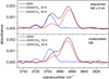 |
Fig. 1. IR spectra of the dangling bond vibrations of water for CH4:H2O mixtures grown at 30 K and warmed to 50 K at 5 K min−1, compared with the spectrum of pure water ice grown at 30 K. Top panel: layered ice (H2O on top of ASW). Bottom panel: co-deposited ice. All spectra correspond to ASW layers of about 200 nm |
On the other hand, the lower panel in Fig. 1 shows the DB features observed when a CH4:H2O ice is grown by simultaneous deposition at 30 K (black trace). In particular, the pure ASW DB feature at 3720 cm−1 and most of the 3696 cm−1 peak (blue trace) are missing in the 30 K co-deposited ice. This indicates that methane molecules already cover most of the ASW pore surface in this kind of mixture. When the mixture is warmed to 50 K, no changes in the DB spectral profile occur, and only a decrease in intensity is observed (red trace). This decrease, similarly to what happened in sequential ices, is due to some CH4 loss, but it also reflects a decrease in the ASW specific surface area. In relation to the overall intensity of the DB features in CH4:H2O co-deposited ices, it should be pointed out that, as described in previous works (Gálvez et al. 2009; Herrero et al. 2010), the DB intensity in the mixtures is always higher than that of the pure ice, and it increases with CH4 concentration.
Most of the water ice reorganisation takes place during the warm up process from 30 K to Tiso; nonetheless, ASW morphology changes may continue during the time elapsed at that Tiso. This is something to be aware of when analysing the experimental data, since it is assumed (see section on diffusion modelling) that methane molecules move through the pore surface of an ASW fix structure. The DB evolution at Tiso might give an idea of the importance of that reorganisation. Figure 2 shows the DB feature for sequential and co-deposited ices at different times during the isothermal experiment. The main spectral variation shown in both panels of Fig. 2 is a decrease in the 3665 cm−1 band, which is associated with CH4 loss. The rest of the DB features suffer from minor modifications, indicating ASW reorganisation is not significant during the isothermal experiment.
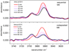 |
Fig. 2. IR spectra of the dangling bond vibrations of water for CH4:H2O mixtures grown at 30 K and warmed to 50 K. Spectra taken at 50 K at different times during the isothermal experiments. Top panel: layered ice (H2O on top of ASW). Bottom panel: co-deposited ice. |
Following the intensity decay of the 1300 cm−1 band, it was possible to quantify the fraction of CH4 that leaves the ice during the heating of the ice mixture via IR spectroscopy. Table 1 displays the CH4/H2O number of molecules ratio at 30 K; at Tiso, at the beginning of isothermal experiment; and at the end of the isothermal experiment. Looking at Cols. 6 and 7, it can be observed that a fraction CH4 is already lost at the beginning of Tiso, which indicates CH4 is distributed through the whole ASW top layer at this time. In comparing Cols. 7 and 8, it can be seen that the fraction of methane that left the ice during the isothermal experiment is small, that is 20% on average. Most methane remains trapped in the ASW structure at the end of the isothermal experiment, both in sequential and in co-deposited ices, as the experiments monitor only the methane that diffuses through the open canals (pores) of this structure. As it is well known from thermal programmed desorption measurements of H2O:CH4 mixtures, a release of methane around 40–50 K is followed by a second desorption peak around 140 K (associated with the amorphous-to-crystalline water phase change, “volcano” desorption), and a last desorption peak appears together with water sublimation, revealing that even a small fraction of CH4 stays in the water ice structure until its sublimation (see, e.g. May et al. 2013).
3.2. Diffusion of CH4 in ASW
3.2.1. Madrid experiments
Figure 3 shows the decay of the intensity of the 1300 cm−1 band of methane versus time elapsed at 50 K for the set of experiments presented in Table 1. The integral has been normalised to the band intensity at the beginning of the isothermal experiment. The panels in the first two rows correspond to sequential deposited ices, with a water ice thickness layer that varies between 145 nm and 480 nm. Panels in the bottom row display the co-deposited ice experiments with an ASW thickness of ∼200 nm. Three isothermal experiments, which were performed at 50 K, 55 K, and 60 K and correspond to layers ∼500 nm thick, are presented in Fig. 4. In order to extract diffusion coefficients from these data, we modelled the decays present in Figs. 3 and 4 using Fick’s second law of diffusion, as is described below in Sect. 3.3.
 |
Fig. 3. Normalised decay of the intensity of the 1300 cm−1 band of CH4 versus time elapsed at 50 K. Diamonds: experimental data. Line: fit to the second Fick diffusion law. |
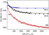 |
Fig. 4. Normalised decay of the intensity of the 1300 cm−1 band of CH4 versus time elapsed at 50 K, 55 K, and 60 K. Scatter points: experimental data. Lines: fit to the second Fick diffusion law. |
3.2.2. Alcoy experiments
Figure 5 presents the variation in the frequency of the QCMB, showing the signal increase, which is proportional to the mass decrease versus the time elapsed at 50 K. In an experiment, the higher the frequency variation is, the higher the fraction of methane molecules that have been sublimated from the ice (Eq. (1)). Frequency variations were scaled to plot these experiments in the same graph. Experiments cover the range of thicknesses studied, between 300 nm and 1000 nm. These experiments have been analysed using Fick’s first law.
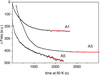 |
Fig. 5. Diffusion of methane from ASW ice grown at 30 K. QCMB signal variation versus time elapsed at 50 K. Black lines: experimental data. Red lines: linear fit employed to derive diffusion coefficients from Fick’s first law. |
3.3. Fickian diffusion modelling
3.3.1. Fick’s second law of diffusion
Fick’s second law of diffusion, which relates the unsteady diffusive flux to the concentration gradient, was applied to obtain the diffusion coefficient, D(T), at a given temperature T. In a one-dimensional system where D(T) does not depend on z, that is, ∂D(T)/∂z = 0, it is given by
 (2)
(2)
where n(z, t) is the concentration of the diffusing species at depth z in the ASW ice at a given time t. Equation (2) is used to describe the methane molecules diffusion along a fixed ASW layer of a known thickness, that is, in a direction perpendicular to the surface substrate. This approach has been shown to give good results to describe similar systems by other authors (Mispelaer et al. 2013; Karssemeijer et al. 2014; Lauck et al. 2015; He et al. 2018). Some initial conditions must be imposed in order to obtain adequate solutions from this equation. It is assumed that all CH4 molecules that reach the surface of the ice layer desorb immediately; therefore, n(L, t) = 0, where L is the ASW ice thickness. Since no CH4 molecules can escape from the bottom of the film, ∂n(0, t)/∂t = 0. As a last condition, the concentration of CH4 is assumed to be homogeneous within the amorphous solid water ice layer at the beginning of the isothermal experiment, n(z, 0) = n0. In particular, for sequential experiments, this last condition implies that during the heating process, methane has diffused into the ASW top layer, filling the pores homogeneously. Sequential experiments were also modelled, imposing a different boundary condition. It was assumed that methane is not homogeneously distributed in the ASW layer, but that it is in a bottom layer while the ASW layer is in top. The fits obtained in this way were worse than those found with the previous approximation. The solutions of Eq. (2) for the constraints of our experiment are (Crank 1975):
 (3)
(3)
where
 (4)
(4)
From these expressions, the column density of methane molecules in the ice can be obtained by integrating the concentration c(z, t) over the ice thickness L. The column density is proportional to the area of a particular CH4 band in the absorbance spectra, A(t), and therefore by integrating over z, the solution can be expressed as (Karssemeijer et al. 2014):
 (5)
(5)
where A0 is the initial band area and s is an offset related to the amount of methane that remains trapped in the ice.
Unweighted least squares fitting of the experimental data presented in Figs. 3 and 4 to Eq. (5) were performed. The solutions are represented with solid lines in the previously mentioned figures. The diffusion coefficients obtained are given in Table 2.
3.3.2. Fick’s first law of diffusion
Fick’s first law describes the relation between the flux of diffusion through a surface and the concentration gradient perpendicular to that surface under steady-state conditions. Fick’s first law is given by
 (6)
(6)
were J is the flux in molec cm−2 s−1, n(z) is the molecular concentration in molec cm−3, and both magnitudes do not change with time.
Isothermal experiments provide the number of methane molecules, n(t), that leave the ice at a particular time. Therefore, it is possible to calculate the methane flow, J(t) = dn(t)/dt. Looking at the final steps of the diffusion experiments, the variation of the flux with time is very slow, and it can be considered almost constant. Then, in that region, Fick’s first law can be applied to extract D(T). Another approximation has to be made in order to estimate the concentration gradient. At times where the methane flow is considered constant, a constant linear distribution of methane through the ASW layer thickness is assumed. The CH4 concentration is expressed as follows: n(z) = a + bz, where n(0) = a at the cold deposition surface, and n(L) = 0 at the ice surface. Consequently, the column density of molecules, N, (molec cm−2) in the ice is given by
 (7)
(7)
From this expression and Fick’s first law, the diffusion coefficient is given by
 (8)
(8)
where L is the ASW layer thickness and J is the methane flow. There is always a fraction of methane molecules that remain trapped in the ice at the end of the diffusion experiments. For the estimation of N, that fraction is not taken into account, and only the CH4 that intervenes in diffusion is considered. To obtain the diffusion coefficients given in Table 2 for the A1–A10 and AA1–AA5 experiments, a linear fit of the QCMB signal at the final part of the isothermal experiments was performed (see Fig. 5). The slope of the fit gives the methane flow that is necessary to derive D(T) with Eq. (8).
4. Discussion of experimental results
Several conclusions can be drawn upon inspecting the results presented in Figs. 3–5 as well as in Table 2. In regards to first and second Fick’s law diffusion coefficients, both approximations give comparable diffusion coefficients, even though Fick’s first law can only be applied to the final part of the isothermal experiments and it imposes stronger restrictions. When both approximations are applied to the same set of experiments (M1–M9), the diffusion coefficients found with the first law are slightly smaller than those found with the second law (see Table 2). The new methodology proposed, based on QCMB detection (exp A1–A10), gives results consistent with those obtained from IR spectrosocopy (M1–M12).
Regarding CH4 diffusion coefficient dependence on ASW ice morphology, the heating ramp affects ASW morphology at Tiso. However, from the inspection of the experiments presented in Table 1, where the ramp was varied between 5 K min−1 and 20 K min−1, it was not possible to extract any conclusion about its effect on methane diffusion. It looks like the morphology variations caused by the different heating ramps are not significant enough to be manifested in the D(T) coefficient.
Upon the inspection of Fig. 3, co-deposited experiments seem to be better described by Fick’s second law than by sequential experiments. Although all fits in Fig. 3 are satisfactory, in order to get proper fits for sequential experiments, only times up to 3000 s were considered. However, co-deposited experiments could be properly fitted in all the experimental time intervals (up to 8000 s). This behaviour is related to differences in the morphology of the ice. Monte Carlo simulations were performed for both ASW structures, pure and co-deposited ASW, shown in Fig. 9 (left panels) and Fig. 10, respectively, illustrating those changes. The diffusion coefficient obtained for co-deposited experiments (M6–M9) vary between 1.4 and 1.8 10−13 cm2 s−1, and those for sequential experiments with a similar layer thickness (M2 and M3) are slightly higher, varying between 2.7 and 3.7 10−13 cm2 s−1. This can be attributed to the effect of methane on ASW porosity upon deposition, since depositing methane together with water slightly decreases the number of pores, slowing the diffusion. This is discussed in Sect. 6.
The D(T) values found for methane diffusing on ASW grown at 50 K (experiments AA1–AA5) are about one order of magnitude smaller than those found for ASW ice grown at 30 K (exp. A5–A8). It is well known that, for background vapour deposition, the higher the growing temperature is, the higher the average density of the ice obtained (Dohnálek et al. 2003), that is, the lower the porosity. Monte Carlo simulations performed in this work corroborate this (see Fig. 9). Consequently, the experimental D(T) values found indicate that CH4 diffuses slower through the pores of the more compact ASW ice.
Pertaining to the ASW ice layer thickness, although unexpected, a dependence of D(T) on the ASW layer thickness was observed in the experiments. All the diffusion coefficients obtained in this work for ASW grown at 30 K and Tiso = 50 K were plotted in Fig. 6 versus the ASW layer thickness. It can be seen that below 600 nm, the fluctuations of diffusion coefficients could be considered within experimental error. However, for layers above 600 nm, there is a clear increase in the diffusion coefficient with thickness. This behavior has been observed by other authors, such as Ghesquière and collaborators (Ghesquière et al. 2015), in analogous experiments performed to study CO2 diffusion in water ice. Also, May and coworkers (May et al. 2013), investigating CH4 diffusion through ASW layers grown on top, conclude that the CH4 releasing mechanism was diffusive only up to a certain ASW layer thickness. A possible reason for observing this behavior could be considering D(T) constant along the z direction within the whole ice layer thickness, as it is assumed in Fick’s law.
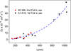 |
Fig. 6. Diffusion coefficient of CH4 at 50 K for different ASW ice layer thicknesses. Red dots: experiments M1–M9. Black squares: experiments A1–A10. Dotted blue line: an exponential fit performed only to help guide the eye. |
Although only a few experiments were performed at temperatures other than 50 K, they could be used to constrain the diffusion barrier, assuming a single-barrier Arrhenius process and a D(T) following Arrhenius equation:
 (9)
(9)
where D0 is the pre-exponential factor, Ed is the diffusion energy barrier, and T is the temperature. With the diffusion coefficients obtained for experiments M3, M4, M10, M11, and M12 at 50, 55, and 60 K, an Arrhenius-type plot was performed to extract a diffusion barrier and pre-exponential factor. Also, experiments AA1–AA5, which give diffusion coefficients at temperatures between 42.5 and 52.5 K for ASW ice grown at 50 K, were fitted to the Arrhenius equation. Both fits are presented in Fig. 7.
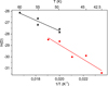 |
Fig. 7. Arrhenius-type plot of the diffusion coefficients of CH4 on ASW grown at 30 K (black triangles) and at 50 K (red dots). |
Energy barriers of 477 ± 91 K and 639 ± 118 K, and pre-exponential factors of ln(D0) = −18 ± 2 (log(D0) = −8.0 ± 0.9) and ln(D0) = −16 ± 3 (log(D0) = −7.0 ± 1.3), were found for both sets of data, which correspond to ASW grown at 30 K and 50 K, respectively. In a previous work, He and coworkers (He et al. 2018) measured the diffusion coefficient of CH4 on ASW grown at 10 K and annealed to 70 K for 30 min. From their experiments, which were performed at temperatures between 17 K and 23 K, they found that Ed = 547 ± 10 K and ln(D0) = −14.3 ± 0.5 (log(D0) = −6.23 ± 2). Their data, compared with those obtained in this work, are presented in Fig. 8. The solid lines represent the extrapolations of the temperature dependence given by the Arrhenius equation. The differences between the three sets of data could be due to differences in the morphology of the ASW ice, which were either grown at 10 K, 30 K, or 50 K.
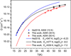 |
Fig. 8. CH4 diffusion coefficients obtained in this work compared with those in (He et al. 2018). Scattered points: experimental data. The temperatures indicated in the legend refer to the ASW generation temperature. Straight lines: fits extracted from Arrhenius plots. |
5. Monte Carlo simulations
We used a step-by-step Monte Carlo simulation to follow the formation of H2O ices with CH4-trapped gas through co-deposition. Our model is described in Cazaux et al. (2015, 2017). We note that H2O and CH4 molecules originating from the gas phase arrive at a random time and location on the substrate, and they follow a random path within the ice. The arrival time depends on the rate at which gas species collide with the surface (Sect. 5.1). The molecules arriving on the surface can be bound to the substrate and to other H2O and CH4 molecules through hydrogen-bound and van der Waals interactions. In the present study, we used on-lattice kinetic Monte Carlo (KMC) simulations. Other types of simulations, such as those using the off-lattice KMC method, have also been used to compute the porosity in ices (Garrod 2013). While this method is more sophisticated than the present method since it allows one to determine the distance of the species explicitly, here, we consider the distance between water molecules to be equal and concentrate on defining the binding energies as a function of neighbours. Because our method does not compute the distance between molecules, the diffusion could be slightly different. However, we can provide diffusion barriers that can be compared with experimental results and used in theoretical models.
In the present study, we consider two distinct cases on how to calculate the binding energies, depending on whether it concerns a water or a methane molecule. For water, the binding energy of each H2O molecule depends linearly on its number of neighbours, as described in Cazaux et al. (2015). For methane, we consider that the binding energy of those molecules is already very high for one neighbour, and very close to the binding energies measured experimentally (Escribano et al., priv. comm.). We therefore consider that the diffusion energy of methane, which is a fraction of the binding energy, does not depend on the number of neighbours, and we use Ed ∼ 550 K, as determined in He et al. (2018). This value was chosen because we compare our experimental results with those of He et al. (2018) (see Sect. 6.3), even though different binding energies appear in the literature (see Luna et al. 2014 and references therein). Depending on their diffusion energies, the H2O and CH4 molecules diffuse on the surface and in the ices. The diffusion is described in Sect. 5.2. While warming up and during the waiting time, the molecules can evaporate from the substrate and ices. In order to reproduce experimental measurements, we deposited water and methane at 30 K with an H2O:CH4 ratio of 10:1. We then increased the temperature after deposition with a ramp of 1 K every 10 s (which is 6 K min−1, providing a ramp close to experimental values ranging between 5 to 10 K per min). When the temperature of 50 K was reached, we let the system evolve with time at a constant temperature and determined the number of molecules evaporating and staying in the ice. This allowed for a direct comparison with the measurements of Sect. 3.
5.1. Accretion
In our model, we defined the surface as a grid with a size of 60 × 60 sites. Low-density amorphous ice mainly consists of four coordinated tetrahedrally ordered water molecules. As already discussed in Cazaux et al. (2015), amorphous water ice is modelled using a grid in which the water molecules are organised as tetrahedrons, which implies that each water molecule has four neighbours. Molecules from the gas-phase arriving on the grid can be bound to the substrate. The accretion rate (in s−1) depends on the density of the species, their velocity, and the cross section of the surface, and it can be written as follows:
 (10)
(10)
 (11)
(11)
where  cm s−1 and
  cm s−1 are the thermal velocity of water and methane, respectively, and σ is the cross section of the surface. Furthermore, S is the sticking coefficient that we consider to be unity in this study. The distance between two sites is 1.58 Å, but each water molecule occupies one site over four because of its four coordinates tetrahedral order (see Cazaux et al. 2015). The surface density of water molecules is what is typically assumed, that is
∼(1/4 × 1.58−2)Å−2 ∼ 1015 cm−2. The cross section scales with the size of the grid are considered in our calculations, with 60 × 60 sites, as σ ∼ (1.58 10−8 × 60)2 cm2 = 9 10−13 cm2. The deposition rate is, therefore, Racc(H2O) = 3 10−8nH2O s−1 and Racc(CH4) = 3.2 10−8nCH4 s−1 for Tgas = 100 K. In order to mimic the experimental conditions with deposition rates of 1 nm s−1 ∼ 6 ML s−1 ∼ 450 molecules s−1 (we have 60 × 60/8 molecules per ML), we set the density of H2O molecules in the gas in cm−3 to nH2O = 9 × 1010 cm−3. The density of CH4 was scaled to the density of water to reproduce the experiments with H2O:CH4 10:1.
cm s−1 are the thermal velocity of water and methane, respectively, and σ is the cross section of the surface. Furthermore, S is the sticking coefficient that we consider to be unity in this study. The distance between two sites is 1.58 Å, but each water molecule occupies one site over four because of its four coordinates tetrahedral order (see Cazaux et al. 2015). The surface density of water molecules is what is typically assumed, that is
∼(1/4 × 1.58−2)Å−2 ∼ 1015 cm−2. The cross section scales with the size of the grid are considered in our calculations, with 60 × 60 sites, as σ ∼ (1.58 10−8 × 60)2 cm2 = 9 10−13 cm2. The deposition rate is, therefore, Racc(H2O) = 3 10−8nH2O s−1 and Racc(CH4) = 3.2 10−8nCH4 s−1 for Tgas = 100 K. In order to mimic the experimental conditions with deposition rates of 1 nm s−1 ∼ 6 ML s−1 ∼ 450 molecules s−1 (we have 60 × 60/8 molecules per ML), we set the density of H2O molecules in the gas in cm−3 to nH2O = 9 × 1010 cm−3. The density of CH4 was scaled to the density of water to reproduce the experiments with H2O:CH4 10:1.
5.2. Diffusion
We used a method to simulate diffusion in a similar way as in Cazaux et al. (2015). The diffusion barrier is usually considered in models as a fraction of the binding energy. For water, the binding energy increases with the number of neighbours and, therefore, the diffusion barrier also increases with the number of neighbours. For CH4, on the other hand, we consider only one binding energy with water. Additionally, that the binding energy does not increase with the number of neighbouring water molecules, which is consistent with the very small differences in binding energies as seen in Luna et al. (2014). The diffusion rate for methane is, therefore, simply  , where ν is the pre-exponential factor and Ed is the diffusion barrier for methane.
For water, we computed the binding energy by adding the number of neighbours nn as Eb = nn × Eb(H2O-H2O), with Eb(H2O-H2O) ∼ 0.2 eV ∼ 2550 K (Brill & Tippe 1967; Isaacs et al. 1999; Dartois et al. 2013) with a pre-exponential factor of 1013 s−1 (Fraser et al. 2001). We defined the diffusion rates by calculating the initial energy of a molecule and its final energy in the possible sites where it can move. For a position (i, j, and k) of a molecule in the grid, we calculated the associated binding energy Ei and identified the possible sites to which the molecule can diffuse as i ± 1, j ± 1, and k ± 1. The final binding energy, Ef, was calculated as a function of the neighbours present around this site. The diffusion rate, from an initial site with an energy of Ei to a final site with an energy of Ef, is illustrated in Cazaux et al. (2017). The barrier to go from Ei to Ef is defined as follows if Ei ≤ Ef:
 (12)
(12)
If Ei > Ef, on the other hand, the barrier becomes:
 (13)
(13)
with ΔE = max(Ei, Ef) − min(Ei, Ef). By defining the barriers in such a manner, we do take microscopic reversibility into account in this study (Cuppen et al. 2013), which implies that barriers that move from one site to another should be identical to the reverse barrier. The diffusion barriers scale with the binding energies with a parameter α. For water, α sets the temperature at which water molecules can re-arrange and diffuse in the ices to form more dense ices. This parameter is found to be around 30% for the water-on-water diffusion derived experimentally (Collings et al. 2003), and we obtained an alpha lower than 40% in a previous study (Bossa et al. 2015). For methane, He et al. (2018) derived a value for α ranging between 34 and 50% and a binding energy ranging from 1100 K to 1600 K. In this study, we use our simulations to constrain the diffusion barrier.
The diffusion rate for water, in s−1, can be written as:
 (14)
(14)
where ν is the pre-exponential factor, T is the temperature of the substrate (water ice or CH4 ice), and Es is the energy of the saddle point, which is Es = (1 − α) × min(Ei, Ef). This formula differs from typical thermal hopping because the energy of the initial and final sites are not identical (Cazaux et al. 2017).
The pre-exponential factor is related with the vibrational frequency of a species in its site, and it can be derived from the following expression of Landau & Lifshitz (1951):  , where Ns is the number of sites per surface area (1015), mCH4 is the mass of methane, and Ei the binding energy. In this work, we have taken ν = 1013 s−1 for water and ν = 109 s−1 for CH4 (He et al. 2018).
5.3. Sublimation
The molecules present on the surface can return into the gas phase because they sublimate. This desorption rate depends on the binding energy of the species with the surface and ice. As mentioned previously, the binding energy of an H2O molecule depends on its number of neighbours, while we consider a unique binding energy for CH4, independent of the number of neighbours. The binding energy Ei of a molecule sets the sublimation rate as:
 (15)
(15)
where ν is the pre-exponential factor, which is taken as ν = 1013 s−1 for water and ν = 109 s−1 for CH4 (He et al. 2018). We used a pre-exponential factor similar to the one used for diffusion for simplicity purposes. However, we also used the lowest binding energy of methane derived from experiments of 1100 K. In this sense, the desorption rate at 30 K is around Rsubl(CH4) = 10−7 s−1, which is similar to a rate with a pre-exponential factor of 1012 and a binding energy of 1300 K. We, therefore, used a sublimation rate in the range of what has been derived in other studies (He et al. 2018). Using a different pre-exponential factor and binding energy for sublimation do not change our results after deposition. Methane molecules desorb once they have diffused through the ice thus reaching the surface and, therefore, our results depend on the diffusion rate rather than the sublimation rate.
6. Theoretical results
6.1. Water ice morphology and porosity
The experiments were performed for a deposition of water and methane at 30 K with a rate of around 1 nm s−1 and a ratio of H2O:CH4 of 10:1. The ice was then heated until 50 K and the diminution of the IR absorbance spectra has given the amount of CH4 desorbing from the ice. Measuring the concentration of CH4 with time can directly give a constraint on the diffusion coefficient, as shown in the previous sections. The CH4 diffuses through the pores within the water ice, which implies that the porosity of water ice could play a role in the diffusion. To grasp how water ice changes within the conditions explored in the present experiments, we show the morphology of water ice with our simulations when deposited at 30 K (Fig. 9, top left panel) and heated at 50 K (Fig. 9, top middle panel), and being deposited at 50 K (Fig. 9, top right panel). At 30 K, the water ice mostly presents water molecules with one and two neighbours as the Fig. 9 (top left) mostly shows blue and green colours. However, when the ice is heated to 50 K, the colour in Fig. 9 (top middle) changes to green and yellow (less blue appears), showing that water molecules did rearrange and molecules with one neighbour moved to another location with more neighbours. If the deposition occurs at 50 K (top right), then the dominating colours are blue and green as in the first figure. This is because this simulation shows the state of the ice just after accretion and molecules are still re-organizing. The bottom panels show the size of the pores in the water ice. These panels are the negative images of the top panels and show the emptiness within the ices. The colour shows the size of the pores, with a minimum of two (blue) to four (yellow). A pore size of two indicates that the two grid cells around the pore are empty, while a size of three or four indicates larger pores of three or four grid cell sizes (in radius). One grid cell represents ∼1.6 Å and, therefore, pores vary from 3.2 to 6.4 Å. The different panels show the network of pores after deposition at 30 K (left panel), after the ice deposited at 30 K having been heated to 50 K (middle panel) and for ice having been deposited at 50 K (right panel). The pores in the case of deposition at 30 K are less and less connected than if the water is subsequently heated to 50 K. The evolution of the network of pores shows how diffusion within the pores takes place when methane is added into the water ice. When water ice is deposited at 50 K, the pores are smaller and less connected, which indicates that diffusion would be less efficient.
 |
Fig. 9. Water morphology and porosity under our experimental conditions. Top panels: water ice being deposited at 30 K (left panel) and then being heated to 50 K (middle panel) and water ice being deposited at 50 K (right panel). Each square represents a water molecule and the colour represents the number of the neighbour for each molecule. Blue squares represent water molecules with one neighbour, green with two neighbours, yellow with three neighbours, and red with four neighbours. Bottom panels: size of the pores in the water ice, which is the negative image of the top panel (showing the emptiness in ice). The colour shows the number of grid cells that are empty around the cell (corresponding to 1.6 Å). The figures show deposition at 30 K (left panel), after being heated to 50 K (middle panel) and being deposited at 50 K (right panel). |
6.2. Methane diffusion in thin water ice: Effect of diffusion barrier and porosity
In order to understand the trapping and diffusion of methane in water ices, we performed Monte Carlo simulations for thin ices deposited at 30 K, which were heated until 50 K and with a waiting time similar to those observed experimentally. Methane was deposited simultaneously with the water, with a ratio of H2O:CH4 of 10:1. In this section, we use thin ices of 10 nm thick to study the effect of the diffusion barriers and of the water ice morphology. In Fig. 10, we illustrate how methane is mixed within water ice in one of our simulations. The ice mixture is represented just after deposition at 30 K. In these simulations, we used a diffusion barrier of Ed = 0.4 Ei for water and a diffusion barrier of Ed = 660 K for methane; it is important to note that for water, Ei depends on the number of neighbours, while the diffusion barrier for methane is always the same. The ice is slightly thicker when methane is included in the simulations. This is due to the fact that at 30 K, methane diffuses as much as water with one neighbour, which implies that the reorganisation is faster than if the ice was composed of 100% water ice. The porosity, presented in Fig. 10 (right panel), seems to be less important than in the case of pure water (bottom left panel in Fig. 9). This could be due to the fact that the molecules do diffuse slightly more than for 100% water, which decreases the coalescence of pores to form networks. It is possible to relate this with the diffusion coefficients found for sequential and co-deposited ices, and this is commented on in Sect. 4. In sequential ices, CH4 diffuses through a pure AWS layer, which is slightly more porous than the ASW generated by co-depositon, and therefore a faster CH4 diffusion is expected.
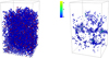 |
Fig. 10. Water ice (blue) with methane (red) after deposition at 30 K (left panel). The right panel shows the size of the pores in the water ice mixed with methane. Pore sizes vary from ∼6 to 10 Å in diameter. |
The effect of the reorganisation of water is illustrated in Fig. 11 (left panel). In this figure, we fixed the diffusion of methane with Ed = 990 K. The diffusion of water was set to two different values of α(H2O) = 0.4 (red) and 0.9 (blue), which gives a diffusion barrier of Ed = α(H2O) Ei. This figure shows that the reorganisation of water has an effect on the diffusion of methane. This is due to the fact that methane diffuses in pores up to the surface of the ice. The reorganisation of water affects the presence of pores and the way they are connected. A slower diffusion of water creates less pores and, consequently, the diffusion of methane is somewhat slower. The diffusion of methane is presented in Fig. 11 (right panel) for Ed = 660 K (red) and 990 K (green). The diffusion of water was set to α(H2O) = 0.4, which gives Ed = 0.4 Ei. A lower mobility of methane (Ed = 990 K) implies that the diffusion is slower and that the amount of methane desorbing from the ices is smaller. This is seen in the figure when comparing this slower diffusion to a faster diffusion given by a smaller barrier of Ed = 660 K. Therefore, both the mobility of water and methane are key parameters to constrain the diffusion coefficient of methane in water ices.
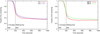 |
Fig. 11. Left panel: effect of water diffusion on the amount of methane remaining in the ice. In red, Ed(H2O) = 0.4 Ei, while in blue, Ed(H2O) = 0.9 Ei. Right panel: effect of methane diffusion on the amount of methane remaining in the ice. In red, Ed(CH4) = 660 K, while in green, Ed(CH4) = 990 K. |
6.3. Thick ice: Constraining the diffusion from experimental data
Most of the experimental measurements that were used to determine the diffusion were obtained on ices with a thickness larger than 180 nm. Our simulations can be made for thin ices, or for thick ices when diffusion is slow, but they cannot be performed for fast diffusion in thick ices due to large computing times. In the present section, we show an alternative solution to simulate the amount of CH4 remaining in thick ices. We made calculations for ices that are 10 nm thick and used several of these thin ices to scale the results to a thick ice. Since we are able to compute the number of CH4 evaporating from a 10 nm ice, we could compute the amount of CH4 evaporating from several blocks of thin ices attached to each other to mimic a thick ice. If the fraction of CH4 evaporating from the 10 nm thick ice is NEVCH4, then the fraction of CH4 evaporating from two blocks of 10 nm thick ice is  (the second term shows the fraction reaching the top block from the bottom block, and then crossing the top block to evaporate). If we would have n blocks of ice attached to each other, we could estimate the fraction of CH4 evaporating as
  . In order to validate our method, we computed the amount of CH4 that stays in the ice with one block of 10 nm, one of 25 nm, and one of 50 nm. The amount of CH4 remaining in the ice was computed for 2 × 25 nm as 1–1/2 × (
 ), where NEVCH4 is the number of CH4 that evaporates from a block that is 25 nm thick, while for 5 × 10 nm as 1–1/5 × (
 ), where NEVCH4 is the amount of CH4 evaporating from a block that is 10 nm thick. The simulations for a 50 nm thick ice along with the simulations for 2 × 25 nm and 5 × 10 nm are shown in Fig. 12. We can see that this method shows very good agreement to estimate the amount of CH4 remaining, with a very small difference on short timescales below 1000 s and a difference of a few percent for larger timescales. We can therefore use this method to reproduce the amount of CH4 remaining in thick ices in the experiments. These simulations were made for slow diffusion where Ed = 990 K for methane and Ed = 0.9 Ei for water.
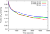 |
Fig. 12. Comparison of the fraction of CH4 remaining for a 50 nm (in blue) compared with the fraction in two blocks of 25 nm attached (red) and five blocks attached (green). |
In the simulations presented in this section, we aim to reproduce the experimental results from Sect. 3 in order to constrain the diffusion coefficient of methane on ASW deposited at 30 K. In our simulations, we used the results obtained in experiment M7 and also used different diffusion rates from He et al. (2018) (mentioned as R1) and the ones derived in this work. We converted the D0 obtained previously with the formula, D0 =  , as shown in He et al. (2018), where ν is the pre-exponential factor, and a = 3 Å is the distance between the two sites. We used the rate derived by He et al. (2018) of R1 = 2 10
 s−1 and the derived rates from the present study, R2 = 4 10
 s−1 and R3 = 4 10
 s−1. We also consider another rate R4 in order to show the effect of the increase in the pre-exponential factor on the fraction of trapped CH4. In this case, R4 = 2 10
 s−1. Figure 13 (left panel) shows the fraction of CH4 remaining after heating, using the rates mentioned above. In the experiments, 0.88 % of methane is still present in the ice when reaching 50 K. Our model cannot account for such a loss with the rates considered. In order to reproduce the measurements, a higher rate (higher ν or lower activation energy) should be used. This implies that in the present case, the diffusion is hindered because many molecules are diffusing back and forth in pores before being able to arrive to the surface and desorb. In other words, the microscopic diffusion of methane is many times faster than the diffusion measured experimentally. Indeed, methane molecules are constantly diffusing within the ices, which can add up to a very long path, while the actual distance travelled is orders of magnitude lower. This is illustrated by Fig. 14, which shows the movement of three methane molecules taken randomly in the ices. The three methane molecules move within the pores without reaching the surface, and the total distance they explored in the ice is very different from the actual path they followed. The symbols show the position of each molecule during the entire simulation. These are the results from simulations using ν = 2 109 s−1 and Ed = 660 K for a 10 nm thick ice. The simulations follow the movement of individual molecules during the heating ramp and waiting time, which lasts ∼1000 s in total. It is important to note that we consider that molecules can move from one side of the box to another, that is to say if a molecule reaches the limit of the box and moves outside, its position is placed to the other side of the box, which happens with the green molecule. Figure 13 (right panel) shows our Monte Carlo results compared to the experimental measurements for a 185 nm thick ice. The simulations overestimate the fraction of CH4 remaining in the ice for the four rates considered. We note that for R4, the calculation is computationally expensive, and we only show the results of the simulations until 2000 s. This implies that to reproduce the experimental results, the diffusion should be faster (higher pre-exponential factors or lower activation energy) than the diffusion obtained using Fick’s law. Our results show that the rates extracted from the present study as well as the rate from He et al. (2018) do not reproduce the experimental data with our Monte Carlo simulations.
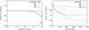 |
Fig. 13. Left panel: fraction of CH4 remaining in the ices during the TPD. The experiments show that 13.8% of CH4 was initially present at 30 K, while 12.1% remained at 50 K. Right panel: fraction of CH4 remaining in the ices during the waiting time after reaching 50 K. The green points show the experimental values. |
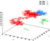 |
Fig. 14. Selection of three methane molecules moving in the grid during the entire experiment. The path clearly illustrates a preferred mobility in the pores. The fact that the green CH4 moves from a side of the box to the other side is due to side effects. |
6.4. Diffusion versus porosity
In this section, we investigate the effect of porosity on the diffusion of methane in the ice. We deposited ices at 30 K and 50 K in our simulations and determined the fraction of methane in the ices as a function of time after 50 K. These results are presented in Fig. 15. For the ices deposited at 30 K, we increased the temperature until 50 K and then determine the amount of CH4 with waiting time; whereas for the ices deposited at 50 K, we determined the amount of CH4 after the deposition was completed. In these simulations, the mobility for water ice was set to Ed = 0.4 Ei for water and Ed = 990 K for methane. We note that for both of the simulations, the diffusion rates are the same and only the deposition temperature changes. Our results show that the porosity changes the diffusion of methane within the ice. A more porous medium, such as the one created when deposition occurs at 30 K, allows for a faster diffusion and therefore less CH4 remains in the ice. On the other hand, a less porous medium, such as the one created when deposition occurs at 50 K, slows down the diffusion and consequently more CH4 molecules remain in the ice. This result is in agreement with experimental findings shown in Fig. 8, where the diffusion coefficient obtained for ices grown at 50 K is smaller (slower diffusion) than the diffusion of ices grown at 30 K. This shows that the porosity plays a role in the diffusion of molecules within the ices and the larger and connected pores favour a higher mobility.
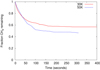 |
Fig. 15. Fraction of methane remaining in the ice after 50 K when deposited at 30 K and at 50 K. |
7. Conclusions
We have investigated the surface diffusion of methane on amorphous solid water and how it is affected by the porosity of the ASW structure. Methane diffusion coefficients have been measured to vary between 10−13 and 10−12 cm2 s−1 for temperatures between 42 K and 60 K. It was observed that different ASW structures modify the CH4 diffusion coefficient up to one order of magnitude.
Experiments and simulations show periods of time where the rate of the sublimation of methane is constant. This implies that the methane concentration gradient remains constant for these time intervals, and the first Fick’s law can be used.
Monte Carlo simulations of simultaneous and sequential H2O:CH4 ices at 30 K show that a more compact ASW structure is formed in co-deposited experiments. The diffusion coefficients measured for CH4 trapped in co-deposited ASW are smaller (slower diffusion) than those found in sequential experiments. Therefore, it is possible to say that when a CH4 reservoir is diffusing through a pure ASW layer that formed on top, the diffusion is faster than in homogeneously mixed H2O:CH4 ices.
Measured diffusion coefficients indicate that CH4 diffuse faster on ices grown at 30 K than in ices grown at 50 K. Monte Carlo simulations show that ices grown at 50 K present smaller and less interconnected pores than ices grown at 30 K. Therefore, it can be concluded that larger and more interconnected pores favour methane diffusion.
We used Monte Carlo simulations in order to better understand the experimental results and to estimate the effect of porosity on the diffusion rates. We show that the diffusion rates derived experimentally using Fick’s laws do not reproduce the experimental results with our Monte Carlo simulations, considering the range of diffusion values within the experimental uncertainty. The experimental results can be reproduced only using a diffusion rate at least 50 times higher, which would imply for the present study a pre-exponential factor ranging between 1010–1011 s−1. They are consistent with factors derived from the expression of Landau & Lifshitz (1951) (see Sect. 5.2). Our work, therefore, shows that the diffusion coefficient obtained from Fick’s law is a diffusion at the macroscopic level. This can be used to determine the overall loss of methane in ices on large timescales, for example when modelling ices of comets or moons. However, when modelling reactivity or ice evolution on the microscopic level with kinetic models (Monte Carlo simulations, rate equations, etc.), the diffusion used should be much higher and the pre-exponential factor can be derived as in Landau & Lifshitz (1951). The discrepancy between a macroscopic (Fick’s law) and microscopic view of diffusion comes from the fact that microscopic models account for back and forth diffusion, counting single diffusion hops in all directions in the medium. In contrast, macroscopic diffusion sees the effective distance that methane molecules travelled, describing CH4 as a continuum medium diffusing due to a concentration gradient. In summary, our work shows that the microscopic diffusion of methane is many times faster than the macroscopic diffusion measured experimentally.
Acknowledgments
Funds from the Spanish MINECO/FEDER FIS2016-77726- C3-1-P and C3-3-P projects are acknowledged.
References
- Berland, B. S., Brown, D. E., Tolbert, M. A., & George, S. M. 1995, Geophys. Res. Lett., 22, 3493 [CrossRef] [Google Scholar]
- Bossa, J., Isokoski, K., Paardekooper, D. M., et al. 2014, A&A, 561, A136 [NASA ADS] [CrossRef] [EDP Sciences] [Google Scholar]
- Bossa, J.-B., Maté, B., Fransen, C., et al. 2015, ApJ, 814, 47 [NASA ADS] [CrossRef] [Google Scholar]
- Brill, R., & Tippe, A. 1967, Acta Crystallogr., 23, 343 [CrossRef] [Google Scholar]
- Cazaux, S., Bossa, J. B., Linnartz, H., & Tielens, A. G. G. M. 2015, A&A, 573, A16 [NASA ADS] [CrossRef] [EDP Sciences] [Google Scholar]
- Cazaux, S., Martín-Doménech, R., Chen, Y. J., Muñoz Caro, G. M., & González Díaz, C. 2017, ApJ, 849, 80 [CrossRef] [Google Scholar]
- Collings, M. P., Dever, J. W., Fraser, H. J., McCoustra, M. R. S., & Williams, D. A. 2003, ApJ, 583, 1058 [NASA ADS] [CrossRef] [Google Scholar]
- Cooke, I. R., Öberg, K. I., Fayolle, E. C., Peeler, Z., & Bergner, J. B. 2018, ApJ, 852, 75 [NASA ADS] [CrossRef] [Google Scholar]
- Crank, J. 1975, The Mathematics of Diffusion, 2nd edn. (Oxford University Press) [Google Scholar]
- Cuppen, H. M., Karssemeijer, L. J., & Lamberts, T. 2013, Chem. Rev., 113, 8840 [CrossRef] [Google Scholar]
- Cuppen, H. M., Walsh, C., Lamberts, T., et al. 2017, Space Sci. Rev., 212, 1 [Google Scholar]
- Dartois, E., Ding, J. J., de Barros, A. L. F., et al. 2013, A&A, 557, A97 [NASA ADS] [CrossRef] [EDP Sciences] [Google Scholar]
- Dohnálek, Z., Kimmel, G. A., Ayotte, P., Smith, R. S., & Kay, B. D. 2003, J. Chem. Phys., 118, 364 [NASA ADS] [CrossRef] [Google Scholar]
- Fraser, H. J., Collings, M. P., McCoustra, M. R. S., & Williams, D. A. 2001, MNRAS, 327, 1165 [NASA ADS] [CrossRef] [Google Scholar]
- Gálvez, Ó., Maté, B., Herrero, V. J., & Escribano, R. 2009, ApJ, 703, 2101 [NASA ADS] [CrossRef] [Google Scholar]
- Garrod, R. T. 2013, ApJ, 778, 158 [NASA ADS] [CrossRef] [Google Scholar]
- Garrod, R. T., Weaver, S. L. W., & Herbst, E. 2008, ApJ, 682, 283 [NASA ADS] [CrossRef] [Google Scholar]
- Ghesquière, P., Mineva, T., Talbi, D., et al. 2015, Phys. Chem. Chem. Phys., 17, 11455 [CrossRef] [Google Scholar]
- Hasegawa, T. I., Herbst, E., & Leung, C. M. 1992, ApJS, 82, 167 [NASA ADS] [CrossRef] [Google Scholar]
- He, J., Emtiaz, S. M., & Vidali, G. 2017, ApJ, 837, 65 [NASA ADS] [CrossRef] [Google Scholar]
- He, J., Emtiaz, S., & Vidali, G. 2018, ApJ, 863, 156 [CrossRef] [Google Scholar]
- He, J., Clements, A. R., Emtiaz, S., et al. 2019, ApJ, 878, 94 [CrossRef] [Google Scholar]
- Herbst, E. 2001, Chem. Soc. Rev., 30, 168 [CrossRef] [MathSciNet] [Google Scholar]
- Herrero, V. J., Gálvez, O., Maté, B., & Escribano, R. 2010, PCCP, 12, 3164 [NASA ADS] [CrossRef] [Google Scholar]
- Irvine, W. M. 2011, Langmuir-Hinshelwood Mechanism (Berlin, Heidelberg: Springer Berlin Heidelberg), 905 [Google Scholar]
- Isaacs, E. D., Shukla, A., Platzman, P. M., et al. 1999, Phys. Rev. Lett., 82, 600 [NASA ADS] [CrossRef] [Google Scholar]
- Jenniskens, P., Blake, D. F., Wilson, M. A., & Pohorille, A. 1995, ApJ, 455, 389 [NASA ADS] [CrossRef] [Google Scholar]
- Karssemeijer, L. J., Ioppolo, S., van Hemert, M. C., et al. 2014, ApJ, 781, 15 [NASA ADS] [CrossRef] [Google Scholar]
- Kerkhof, O., Schutte, W. A., & Ehrenfreund, P. 1999, A&A, 346, 990 [Google Scholar]
- Landau, L. D., & Lifshitz, E. M. 1951, Statistical Physics (Elsevier) [Google Scholar]
- Lauck, T., Karssemeijer, L., Shulenberger, K., et al. 2015, ApJ, 801, 118 [NASA ADS] [CrossRef] [Google Scholar]
- Livingston, F. E., Smith, J. A., & George, S. M. 2002, J. Phys. Chem. A, 106, 6309 [CrossRef] [Google Scholar]
- Luna, R., Satorre, M. Á., Domingo, M., Millán, C., & Santonja, C. 2012, Icarus, 221, 186 [CrossRef] [Google Scholar]
- Luna, R., Satorre, M. Á., Santonja, C., & Domingo, M. 2014, A&A, 566, A27 [NASA ADS] [CrossRef] [EDP Sciences] [Google Scholar]
- Mastrapa, R. M., Sandford, S. A., Roush, T. L., Cruikshank, D. P., & Ore, C. M. D. 2009, ApJ, 1347 [NASA ADS] [CrossRef] [Google Scholar]
- Maté, B., Molpeceres, G., Tanarro, I., et al. 2018, ApJ, 861, 61 [CrossRef] [Google Scholar]
- May, R. A., Smith, R. S., & Kay, B. D. 2013, J. Chem. Phys., 138 [Google Scholar]
- Mispelaer, F., Theulé, P., Aouididi, H., et al. 2013, A&A, 555, A13 [NASA ADS] [CrossRef] [EDP Sciences] [Google Scholar]
- Molpeceres, G., Satorre, M. Á, Ortigoso, J., et al. 2017, MNRAS, 466, 1894 [CrossRef] [Google Scholar]
- Narten, A. H., Venkatesh, C. G., & Rice, S. A. 1976, J. Chem. Phys., 64, 1106 [NASA ADS] [CrossRef] [Google Scholar]
- Raut, U., Teolis, B. D., Loeffler, M. J., et al. 2007, J. Chem. Phys., 126 [Google Scholar]
- Tielens, A. G. G. M., & Hagen, W. 1982, A&A, 114, 245 [Google Scholar]
All Tables
CH4 diffusion coefficients on ASW grown at 30 K (M1–M12 and A1–A10) or at 50 K (AA1–AA5), obtained with two different approximations, Fick’s second law or Fick’s first law, as indicated.
All Figures
|
Fig. 1. IR spectra of the dangling bond vibrations of water for CH4:H2O mixtures grown at 30 K and warmed to 50 K at 5 K min−1, compared with the spectrum of pure water ice grown at 30 K. Top panel: layered ice (H2O on top of ASW). Bottom panel: co-deposited ice. All spectra correspond to ASW layers of about 200 nm |
| In the text | |
|
Fig. 2. IR spectra of the dangling bond vibrations of water for CH4:H2O mixtures grown at 30 K and warmed to 50 K. Spectra taken at 50 K at different times during the isothermal experiments. Top panel: layered ice (H2O on top of ASW). Bottom panel: co-deposited ice. |
| In the text | |
|
Fig. 3. Normalised decay of the intensity of the 1300 cm−1 band of CH4 versus time elapsed at 50 K. Diamonds: experimental data. Line: fit to the second Fick diffusion law. |
| In the text | |
|
Fig. 4. Normalised decay of the intensity of the 1300 cm−1 band of CH4 versus time elapsed at 50 K, 55 K, and 60 K. Scatter points: experimental data. Lines: fit to the second Fick diffusion law. |
| In the text | |
|
Fig. 5. Diffusion of methane from ASW ice grown at 30 K. QCMB signal variation versus time elapsed at 50 K. Black lines: experimental data. Red lines: linear fit employed to derive diffusion coefficients from Fick’s first law. |
| In the text | |
|
Fig. 6. Diffusion coefficient of CH4 at 50 K for different ASW ice layer thicknesses. Red dots: experiments M1–M9. Black squares: experiments A1–A10. Dotted blue line: an exponential fit performed only to help guide the eye. |
| In the text | |
|
Fig. 7. Arrhenius-type plot of the diffusion coefficients of CH4 on ASW grown at 30 K (black triangles) and at 50 K (red dots). |
| In the text | |
|
Fig. 8. CH4 diffusion coefficients obtained in this work compared with those in (He et al. 2018). Scattered points: experimental data. The temperatures indicated in the legend refer to the ASW generation temperature. Straight lines: fits extracted from Arrhenius plots. |
| In the text | |
|
Fig. 9. Water morphology and porosity under our experimental conditions. Top panels: water ice being deposited at 30 K (left panel) and then being heated to 50 K (middle panel) and water ice being deposited at 50 K (right panel). Each square represents a water molecule and the colour represents the number of the neighbour for each molecule. Blue squares represent water molecules with one neighbour, green with two neighbours, yellow with three neighbours, and red with four neighbours. Bottom panels: size of the pores in the water ice, which is the negative image of the top panel (showing the emptiness in ice). The colour shows the number of grid cells that are empty around the cell (corresponding to 1.6 Å). The figures show deposition at 30 K (left panel), after being heated to 50 K (middle panel) and being deposited at 50 K (right panel). |
| In the text | |
|
Fig. 10. Water ice (blue) with methane (red) after deposition at 30 K (left panel). The right panel shows the size of the pores in the water ice mixed with methane. Pore sizes vary from ∼6 to 10 Å in diameter. |
| In the text | |
|
Fig. 11. Left panel: effect of water diffusion on the amount of methane remaining in the ice. In red, Ed(H2O) = 0.4 Ei, while in blue, Ed(H2O) = 0.9 Ei. Right panel: effect of methane diffusion on the amount of methane remaining in the ice. In red, Ed(CH4) = 660 K, while in green, Ed(CH4) = 990 K. |
| In the text | |
|
Fig. 12. Comparison of the fraction of CH4 remaining for a 50 nm (in blue) compared with the fraction in two blocks of 25 nm attached (red) and five blocks attached (green). |
| In the text | |
|
Fig. 13. Left panel: fraction of CH4 remaining in the ices during the TPD. The experiments show that 13.8% of CH4 was initially present at 30 K, while 12.1% remained at 50 K. Right panel: fraction of CH4 remaining in the ices during the waiting time after reaching 50 K. The green points show the experimental values. |
| In the text | |
|
Fig. 14. Selection of three methane molecules moving in the grid during the entire experiment. The path clearly illustrates a preferred mobility in the pores. The fact that the green CH4 moves from a side of the box to the other side is due to side effects. |
| In the text | |
|
Fig. 15. Fraction of methane remaining in the ice after 50 K when deposited at 30 K and at 50 K. |
| In the text | |
Current usage metrics show cumulative count of Article Views (full-text article views including HTML views, PDF and ePub downloads, according to the available data) and Abstracts Views on Vision4Press platform.
Data correspond to usage on the plateform after 2015. The current usage metrics is available 48-96 hours after online publication and is updated daily on week days.
Initial download of the metrics may take a while.