| Issue |
A&A
Volume 642, October 2020
|
|
|---|---|---|
| Article Number | A50 | |
| Number of page(s) | 11 | |
| Section | Planets and planetary systems | |
| DOI | https://doi.org/10.1051/0004-6361/202038703 | |
| Published online | 02 October 2020 | |
Obliquity measurement and atmospheric characterisation of the WASP-74 planetary system★
1
Instituto de Astrofísica de Canarias (IAC),
38205
La Laguna,
Tenerife,
Spain
e-mail: rluque@iac.es
2
Departamento de Astrofísica, Universidad de La Laguna (ULL),
38206,
La Laguna
Tenerife,
Spain
3
Key Laboratory of Planetary Sciences, Purple Mountain Observatory, Chinese Academy of Sciences,
Nanjing
210023,
PR China
4
Department of Astronomy, The University of Tokyo 7-3-1, Hongo, Bunkyo-ku,
Tokyo,
113-0033,
Japan
5
Science Support Office, Directorate of Science, European Space Research and Technology Centre (ESA/ESTEC), Keplerlaan 1,
2201
AZ Noordwijk,
The Netherlands
6
Department of Earth and Planetary Science, Graduate School of Science, The University of Tokyo, 7-3-1 Hongo, Bunkyo-ku,
Tokyo
113-0033,
Japan
7
SRON Netherlands Institute for Space Research, Sorbonnelaan 2,
3584 CA
Utrecht, The Netherlands
8
Institute of Planetary Research, German Aerospace Center, Rutherfordstrasse 2,
12489
Berlin,
Germany
9
Astrobiology Center of NINS, 2-21-1, Osawa, Mitaka,
Tokyo
181-8588,
Japan
10
National Astronomical Observatory of Japan, 2-21-1 Osawa, Mitaka,
Tokyo
181-8588,
Japan
11
Komaba Institute for Science, The University of Tokyo, 3-8-1 Komaba, Meguro,
Tokyo
153-8902,
Japan
12
JST, PRESTO, 3-8-1 Komaba, Meguro,
Tokyo
153-8902,
Japan
13
Department of Astronomical Science, The Graduated University for Advanced Studies, SOKENDAI, 2-21-1, Osawa, Mitaka,
Tokyo
181-8588
Japan
Received:
19
June
2020
Accepted:
22
July
2020
We present new transit observations of the hot Jupiter WASP-74 b (Teq ~ 1860 K) using the high-resolution spectrograph HARPS-N and the multi-colour simultaneous imager MuSCAT2. We refined the orbital properties of the planet and its host star and measured its obliquity for the first time. The measured sky-projected angle between the stellar spin-axis and the orbital axis of the planet is compatible with an orbit that is well-aligned with the equator of the host star (λ = 0.77 ± 0.99 deg). We are not able to detect any absorption feature of Hα or any other atomic spectral features in the high-resolution transmission spectra of this source owing to low S/N at the line cores. Despite previous claims regarding the presence of strong optical absorbers such as TiO and VO gases in the atmosphere of WASP-74 b, new ground-based photometry combined with a reanalysis of previously reported observations from the literature show a slope in the low-resolution transmission spectrum that is steeper than expected from Rayleigh scattering alone.
Key words: planetary systems / planets and satellites: individual: WASP-74 b / planets and satellites: atmospheres / methods: observational / techniques: photometric / techniques: radial velocities
Light curve data are only available at the CDS via anonymous ftp to cdsarc.u-strasbg.fr (130.79.128.5) or via http://cdsarc.u-strasbg.fr/viz-bin/cat/J/A+A/642/A50
© ESO 2020
1 Introduction
Metal oxides, such as TiO and VO, have been proposed to exist in the atmospheres of highly irradiated hot Jupiters introducing thermal inversions in the temperature structure (Hubeny et al. 2003; Fortney et al. 2008). However, these early theoretical predictions have barely been confidently confirmed by observations. The overall lack of TiO/VO detections in optical transmission spectroscopy then triggered several alternative theoretical interpretations such as TiO/VO condensation (Spiegel et al. 2009), stellar activity (Knutson et al. 2010), or high C/O ratio (Madhusudhan 2012).
The progress first appeared in the emission spectroscopy of so-called ultra-hot Jupiters (UHJs; Parmentier et al. 2018), which are defined as gas giants with dayside temperatures hotter than ~2200 K. Both low- and high-resolution emission spectra of the UHJ WASP-33 b indicate the presence of TiO in its dayside atmosphere (Haynes et al. 2015; Nugroho et al. 2017). Later, both transmission and emission spectroscopy of another UHJ, WASP-121 b, revealed that the VO molecule is present in its atmosphere (Evans et al. 2016) and is responsible for the observed thermal inversion (Evans et al. 2017). But the original tentative inference of TiO by multi-band photometry (Evans et al. 2016) was later ruled out by low-resolution transmission spectroscopy (Evans et al. 2018). The first significant detection of TiO in the optical transmission spectrum came from the UHJ WASP-19 b (Sedaghati et al. 2017), although this has not been confirmed by another independent work, suggesting that stellar contamination could introduce false positive TiO signatures (Espinoza et al. 2019). The search for TiO/VO in the optical transmission spectroscopy remains unresolved. An alternative explanation is that Fe is responsible for the thermal inversion, a claim that is gaining support with the recent detection of Fe I in the emission spectra of two UHJs, KELT-9 b (Pino et al. 2020) and WASP-189 b (Yan et al. 2020).
We present a study of the system WASP-74 (Hellier et al. 2015) using multi-colour photometry and high-resolution spectroscopy observations with the Multicolour Simultaneous Camera for studying Atmospheres of Transiting exoplanets (MuSCAT2) and High Accuracy Radial velocity Planet Searcher in North hemisphere (HARPS-N), respectively. WASP-74 b is a hot Jupiter in a two-day orbit around a F9 star with a magnitude V = 9.75 mag. With an equilibrium temperatureof around 1900 K, this planet remains very close to the UHJs region. Tsiaras et al. (2018) and Mancini et al. (2019) measured its transmission spectra using the Wide Field Camera 3 (WFC3) on board the Hubble Space Telescope (HST) and ground-based multi-band photometry,respectively. Their findings, although tentative, indicate a water-depleted atmosphere with strong optical absorbers such as TiO and VO. We revise these findings with our new observations and a reanalysis of the previously published data.
Moreover, the time series of high-resolution data during a transit allows us to investigate the architecture of the planetary system. During a transit, the planet blocks a moving portion of the stellar disc and the corresponding RV of that stellar region is masked from the integrated stellar RV. This generates a RV anomaly during the transit, which is known as the Rossiter-McLaughlin (RM; Rossiter 1924; McLaughlin 1924) effect. The RM signal has been used to estimate the projected spin-orbit angle (λ), the angle between the normal vector of the orbital plane, and the stellar rotational spin-axis. So far a wide diversity of spin-orbit angles have been measured, ranging from aligned (Winn 2010) to highly misaligned systems (Addison et al. 2018), and even retrograde planets (e.g. Hébrard et al. 2011). An statistically large sample of spin-orbit angle is essential to examine theories on planet formation and evolution (e.g. Winn et al. 2005; Triaud et al. 2010; Albrecht et al. 2012; Triaud 2017). For instance, Winn et al. (2010) found that hot Jupiters have larger spin-orbit angles if they are orbiting hot stars (Teff > 6100 K). Several explanations were proposed for this trend, connecting it to the star-planet tides that can align the planetary orbits with the stellar equator; tides should be stronger for cooler stars. In this work, we find that the WASP-74 spin orbit measurement is in line with this trend.
This paper is organised as follows. In Sect. 2 we describe the multi-colour photometry and high-resolution spectroscopy observations. In Sect. 3 we present the determination of the stellar parameters of the host star. In Sect. 4 we describe the retrieval of the spin orbit alignment of the system via RM measurements. In Sect. 5 we analyse the atmosphere of the planet combining the photometric and spectroscopic data and discuss the absence of TiO/VO and the presence of Rayleigh scattering. Finally, in Sect. 6 we present the summary of our results and conclusions.
Observing log of the WASP-74 b transit observations.
2 Observations
2.1 Multi-colour photometry
We observed four transits (three full, one partial) of WASP-74 b with the MuSCAT2 multi-colour imager (Narita et al. 2019) installed in Telescopio Carlos Sánchez (TCS) located at the Teide Observatory in Tenerife, Spain. Observations were carried out simultaneously in four colours (g, r, i, z) in the three full transits (2018-07-17, 2018-08-16, and 2018-08-31) and only in three colours (g, r, i) for the partial transit (2019-06-24) with a pixel scale of 0.44′′ pix−1. The z-band observations are missing in this transit as a result of a problem with its charged coupled device (CCD), which was under maintenance. A summary of the key properties for each of the nights is presented in Table 1.
The reduction of the multi-colour photometry data was performed with a dedicated MuSCAT2 pipeline including bias and flat-field corrections. In a nutshell, this pipeline calculates aperture photometry for a set of comparison stars and photometry aperture sizes, and creates the final relative light curves via global optimisation of the posterior density for a model consisting of a transit model (with quadratic limb-darkening coefficients), apertures, comparison stars, and a linear baseline model with the airmass, seeing, x- and y-centroid shifts, and the sky level as covariates (see Parviainen et al. 2019 for details).
Mancini et al. (2019) collected broadband photometry in several filters of WASP-74 b to determine the observational transmission spectrum of the planet. Their dataset comprises a total of 18 light curves from 11 different transits between 2015 and 2017 in the following passbands: Bessell U, Johnson B, Sloan g′, r′, i′, and z′, Bessell I, Cousins I, and near-infrared J, H, and K bands. Observations were carried out by the following telescopes: the Calar Alto 1.23 m telescope (one transit in Johnson B and another in Cousins I), Danish 1.54 m telescope (seven transits in Bessell I and two more in Bessell U), and the Gamma-Ray Burst Optical/Near-Infrared Detector (GROND) multi-colour imager at the MPG 2.2 m telescope in La Silla, Chile (one transit in g′, r′, i′, z′, J, H, and K). WASP-74 b was also observed with the HST/WFC3 camera by Tsiaras et al. (2018) for measuring the transmission spectra of a sample of hot Jupiters from 1.1 to 1.7 μm and with Spitzer/IRAC in 3.6 and 4.5 μm (PI: Deming) for a statistical study of secondary eclipses of hot Jupiters by Garhart et al. (2020).
While we used the HST observations as presented in Tsiaras et al. (2018), we performed our own photometric analysis of the Spitzer observations. As in Livingston et al. (2019), we extracted the Spitzer light curves following the approach taken by Knutson et al. (2012) and Beichman et al. (2016) and selected the circular aperture size that minimises the combined uncorrelated and correlated noise (2.2 pix), as measured by the standard deviation and β factor (Pontet al. 2006; Winn et al. 2008). Then, we jointly modelled the transit and systematics inherent to the Spitzer light curves usingthe pixel-level decorrelation method (Deming et al. 2015), which uses a linear combination of (normalised) pixel light curves to model the effect of point-spread function (PSF) motion on the detector coupled with intra-pixel gain variations.
2.2 High-resolution spectroscopy
Three transits of WASP-74 b were observed using the HARPS-N spectrograph (Mayor et al. 2003; Cosentino et al. 2012), mounted on the 3.58 m Telescopio Nazionale Galileo (TNG), located at the Observatorio del Roque de los Muchachos in La Palma, Spain. Two of these were simultaneously observed with MuSCAT2. The HARPS-N spectograph covers the optical wavelength regime between 0.38 and 0.69 μm with a spectral resolution of  . The observations were performed exposing continuously before, during, and after the transit, using an exposure time of 600 s. The signal-to-noise (S/N), calculated as an average of the S/N per pixel in the Na I order (590 nm), ranges from 55 to 88 in the second night and 32 to 64 in the first and third nights. In all three cases, we used fibre B to monitor possible sky emission during the night. Details on the observations are presented in Table 1.
The HARPS-N observations were reduced using the HARPS-N data reduction software (DRS), version 3.7 (Cosentino et al. 2014; GAPS Collaboration 2014). After computing the wavelength calibration solution, the DRS combines and resamples the two-dimensional echelle spectra with wavelength step of 0.01 Å into a one-dimensional spectrum. The final spectra are referred to the barycentric rest frame and standard air wavelengths are used.
3 Stellar parameters
We used the Zonal Atmospheric Stellar Parameters Estimator (ZASPE; Brahm et al. 2017) code to determine the atmospheric stellar parameters of WASP-74. The parameters were obtained with a high S/N spectrum built by co-adding all HARPS-N out-of-transit observations. In summary, ZASPE matches the observed stellar spectrum via least-squares minimisation against a grid of synthetic spectra in the spectral regions most sensitive to changes in Teff, log g⋆, and [Fe/H].Then, to derive the physical parameters of the star, we used PARAM 1.31, a web interface for Bayesian estimation of stellar parameters using the PARSEC isochrones from Bressan et al. (2012). The required inputs are the effective temperature and metallicity of the star determined spectroscopically together with its apparent visual magnitude and parallax.
We derive an effective temperature of Teff = 5883 ± 57 K, a stellar mass of M⋆ = 1.236 ± 0.026 M⊙, and a radiusof R⋆ = 1.444 ± 0.044 R⊙, in fairly good agreement with the most up-to-date values reported in Mancini et al. (2019). The stellar models constrain the age of the star to be 3.49 ± 0.65 Gyr. We stress that the uncertainties on the derived parameters are internal to the stellar models used and do not include systematic uncertainties related to input physics. All derived values and previous values reported in the literature can be found in Table 2.
4 Planetary obliquity
The radial velocities (RVs) of the three nights were computed via serval (Zechmeister et al. 2018), which uses least-squares fitting with a high S/N template to compute the RVs. The template is created by co-adding all the out-of-transit spectra of the star. The RM effect is clearly observed in the extracted RVs of each individual night (Fig. 1).
In order to measure the obliquity (λ) of the system, we fit a RM model to the RV data via the Markov chain Monte Carlo (MCMC) algorithm implemented in emcee (Foreman-Mackey et al. 2013). We used two different RV contributions to build our model: the RM effect and a circular orbit. Both models are implemented in PyAstronomy (Czesla et al. 2019) as modelSuite.RmcL and modelSuite.radVel, respectively. The model containing the RM effect depends on the orbital period (P), transit epoch (T0), planet-to-star radius ratio (Rp ∕R⋆ ≡ k), angular rotation velocity of the host star (Ω), linear limb-darkening coefficient (ɛ), inclination of the orbit (i), inclination of the stellarrotation axis (I⋆), sky-projected angle between the stellar rotation axis, the normal of planetary orbit plane (λ), and the scaled semi-major axis (a∕R⋆ ≡ as). On the other hand, the circular orbit RV contribution depends on P, Tc, the stellar velocity semi-amplitude (K⋆), and the offset with respect to the null RV (γ).
As presented in previous studies (e.g. Casasayas-Barris et al. 2017), in the fitting procedure, I⋆ to 90 deg, while T0, as, k, and R⋆ are fixed to the values derived in Sects. 3 and 5.1. The other parameters (Ω, ɛ, λ, K⋆ and γ) remain free. The RV information from the three nights is jointly fitted, considering that T0, Ω, ɛ, λ are shared parameters. On the other hand, the offset between the model and data (γ) can vary from night to night as, additionally to the system velocity, the RV information is given with possible instrumental and stellar activity effects. The parameter K⋆ could also be affected by activity and become different for different nights (Oshagh et al. 2018). For this reason, we fit one different γ and K⋆ per night (called γ1, γ2, γ3 and K⋆,1, K⋆,2, K⋆,3, respectively).
We analysed the system using 50 walkers and a total of 106 steps and checked their convergence using the Gelman-Rubin statistic. Adequate convergence was considered when the Gelman-Rubin potential scale reduction factor dropped to within 1.03. Each step is initialised at a random point near the measured values from literature. The quantity λ is constrained to ±180 deg, ɛ between 0.5 and 1.0; using ldtk (Parviainen & Aigrain 2015), we estimate a linear limb-darkening coefficient of 0.71 in the HARPS-N wavelength coverage. The quantity Ω is constrained between 0.3 and 0.9 rad d−1, which is translated to v sin I⋆ limited between 3.7 and 11.1 km s−1; Mancini et al. (2019) measured a v sin I⋆ = 6.03 km s−1. The medianvalues of the posteriors are adopted as the best-fit values, and their error bars correspond to the 1σ statistical errors at the corresponding percentiles. The individual RM curves can be observed in Fig. 1. The detrended data of all nights with the best-fit model are presented in Fig. 2. Table 3 shows the posteior distributions of the fitted parameters in the RM joint model.
With the joint fit of the three nights, we measure a spin-orbit angle of 0.8 ± 1.0 deg, meaning analigned system. The angular rotation velocity is measured to be of 0.50 ± 0.04 rad d−1 and v sin I⋆ = 5.85 ± 0.50 km s−1, consistent with our spectroscopically derived results from Table 2 and with the results obtained by Mancini et al. (2019). The v sin I⋆ value derived from the RM fitting differs less than 2σ from Hellier et al. (2015) results. Also, the K⋆ values of the individual nights are consistent among themselves and with the value reported in Hellier et al. (2015), pointing to a low level of stellar activity (Oshagh et al. 2018). This is supported by the absence of spot-crossing events in the MuSCAT2 simultaneous multi-colour photometric observations during HARPS-N first and third transits. Although we cannot assess the impact associated with un-occulted spots affecting both RM and transit observations, we can be confident that our λ and v sin I⋆ determinations are not significantly mis-estimated. There are two reasons supporting this claim; first the results obtained with the joint fit are consistent with the results obtained when fitting each night independently. Second combining three RMs, as was demonstrated in Oshagh et al. (2018), is sufficient to mitigate and minimise the influence of stellar activity on the estimated λ and v sin I⋆. However, aspresented in Cegla et al. (2016) and Bourrier et al. (2017), the spin-orbit and v sin I⋆ measurements performed using the classical RM could be significantly biased due to variations in the shape of the local cross-correlation functions (CCFs).
In Fig. 3 we show the obliquity measurements for known transiting planets (from TEPCat orbital obliquity catalogue; Southworth 2011) with respect to the effective temperature of their host stars. As presented in Winn et al. (2010), we confirm that most of the planets orbiting stars with effective temperatures lower than ~ 6200 K are in aligned systems, while those planets orbiting hotter stars tend to form misaligned systems with a higher frequency. In this context, the WASP-74 system is in agreement with this trend, located at the low-obliquity region. As explained in this same study, this could be the result of the interaction between the planetary orbit inside the convective zone of cool stars; which, owing to tidal dissipation, realign the star-planet system.
Stellar parameters of WASP-74.
Estimates for the system parameters derived from RM effect analysis.
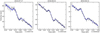 |
Fig. 1 Stellar RVs of WASP-74 for each individual night. The RV measurements are shown in black dots. The best-fit model obtained with the MCMC procedure is shown in cyan. |
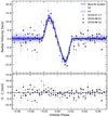 |
Fig. 2 Rossiter-McLaughlin effect during the transit of WASP-74 b after being detrended (top panel), and residuals between the data and model (bottom panel). The RVs from the three different data sets are shown with different symbols. The dark blue line corresponds to the best-fit RM model. The 1σ and 3σ uncertainties of the model are indicated in light blue. |
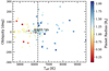 |
Fig. 3 Measurements of orbital obliquity for the known transiting extrasolar planetary systems and brown dwarf companions in front of the effective temperature of the host star (dots), extracted from TEPCat orbital obliquity catalogue (Southworth 2011). The planetary radius is presented in the colour bar. The star symbol corresponds to the spin-orbit measurement of WASP-74 b. The black-dashed vertical line denotes the 6250 K effective temperature transition from Winn et al. (2010). |
5 Atmospheric characterisation
5.1 Multi-colour light curve analysis
We modelled the three full transits from MuSCAT2 jointly with the two Spitzer/IRAC (3.6 and 4.5 μm channels), seven GROND (Sloan g′, r′, i′, z′, J, H, and K passbands), seven Danish 1.54 m Telescope (Bessell I passband), and one Calar Alto 1.23-m(Cousins I passband) light curves presented in Mancini et al. (2019)2. We excludedthe two Danish Bessell U light curves owing to their short pre- and post-transit baselines and strong correlated noise that cannot be sufficiently accounted for using the data available. We also excluded the CA Johnson B light curve because of partial transit coverage; we include partial transits only when we have light curves with full transit coverage in the same passband.
We carried out the light curve analysis of the data in a Bayesian framework following Parviainen (2018). First, we constructed a flux model to reproduce both the transit and the light curve systematics. Then, we defined a noise model to incorporate possible stochastic variability in the observations and combined it with the flux model and the observations to define the likelihood. Using MCMC sampling, we estimated the joint parameter posterior distributions after defining the priors on the model parameters. The analyses were carried out with a custom Python code based on PyTransit (Parviainen 2015), LDTk (Parviainen & Aigrain 2015), emcee (Foreman-Mackey et al. 2013), and other standard Python libraries for astrophysics and scientific computing.
The four parameters describing the orbital geometry of the planet (zero epoch T0, orbital period P, stellar density ρ⋆, and impact parameter b) are independent of passband or per-light-curve systematics, and thus all the light curves constrain the posterior distributions of these parameters. The radius ratio k and the limb-darkening coefficients are wavelength dependent, and thus all the light curves observed in a given passband constrain the posterior densities of these parameters in that passband. Finally, systematics were modelled using a linear combination of state vectors, where the number of covariates varies from dataset to dataset; in most cases at least airmass and x- and y- centroid shifts are available. Each covariate is associated with a free coefficient, and the coefficient posteriors are constrained only by the information in the light curve modelled by the covariate.
We have 11 separate passbands (g, r, i, Cousins I, Johnson I, z, J, H, K, 3.6 μm, and 4.5 μm), so we end up with 11 radius ratio parameters and 22 parameters for the quadratic stellar limb-darkening model. The area ratios have wide uniform priors that do not constrain the posterior, but the limb-darkening coefficients have loosely constraining normal priors created using LDTk (the LDTk-derived prior standard deviation is multiplied by 10) for all the passbands except J, H, and K. We set uniform priors for those passband limb-darkening coefficients that constrain the coefficients to smaller values than the LDTk-derived prior for thez band.
The linear baseline model contributes 105 free parameters to the model in total. The MuSCAT2 light curves have four covariates each (airmass, x- and y-shifts, and aperture entropy that works as a proxy for the full witdh at half maximum) and the GROND light curves have five covariates each (x- and y-shifts, x- and y-FWHMs, and airmass). The publicly available Danish 1.54 m and Calar Alto 1.23 m light curves do not include covariate information.
We first analysed the MuSCAT2 data and GROND data separately to test whether the two datasets agree with each other, and then ran the analysis using the MuSCAT2, GROND, Danish, Calar Alto, and Spitzer light curves jointly; the DK and CA light curves in I band cannot be directly compared with MuSCAT2 and GROND i filter owing to broader wavelength coverage. The MuSCAT2 analysis agrees well with the GROND analysis, although the radius ratio posteriors of the GROND data have larger uncertainties that can be attributed to a passband-dependent instrumental effect (discontinuity) very close to the transit centre that cannot be sufficiently modelled by the linear baseline model. We adopt the results from the full joint analysis as our final result and present them in Table 4, and we also plot all the light curves in Fig. 4.
5.2 Low-resolution transmission spectrophotometry
Multi-colour observations of hot Jupiters can be used to construct a transmission spectrum, which is valuable to probe their atmospheresat the terminator. Figure 5 shows the measured radius ratio in various passbands from the new MuSCAT2 observations together with our reanalysis of the observations from Spitzer, Mancini et al. (2019), and the Tsiaras et al. (2018) HST observations. Our results disagree with those from Mancini et al. (2019, see their Figs. 8 and 9). We find no evidence of TiO/VO in the atmosphere of WASP-74 b, but a steep slope in the optical transmission spectrum.
We attribute the origin of this disagreement to different analyses of the light curves. First, we fit each the available light curves as a function of passband jointly, which constrains the geometry and limb-darkening parameters better than modelling the light curves individually. Second, some of the GROND covariates are relatively noisy and contain a significant amount of strong outliers (especially the centroid estimates in the NIR passbands). Linear baseline models (the approach used also by Mancini et al. 2019) do not perform well with noisy covariates, so we remove the photometry points in which the covariates are clearly problematic; that is, we removed part of the data based on the covariates, but not on the photometry itself. This approach improves the baseline model significantly, and the separate MuSCAT2 and GROND analyses agree well with each other.
We used the PLanetary Atsmopheric Transmission for Observer Noobs code PLATON3 (Zhang et al. 2019) to retrieve the atmospheric properties of WASP-74 b. The PLATON code is a fast, user-friendly open-source code for retrieval and forward modelling of exoplanet atmospheres written in Python. For our retrieval analysis, we assumed an isothermal atmosphere and did not take into account any contamination from stellar heterogeneities (e.g. Oshagh et al. 2014; Rackham et al. 2018, 2019). We fit the combined transmission spectrum, including the low-resolution HST/WFC3 spectrum from Tsiaras et al. (2018), reanalysed Cousins I, Bessell I, and GROND measurements from Mancini et al. (2019), and our new MuSCAT2 and Spitzer measurements. The free parameters are isothermal temperature T, the radius of a planet at a pressure of 1 bar R1bar, C/O ratio, atmospheric metallicity relative to the solar value log Z∕Z⊙, scattering slope s, scattering amplitude log fscatter, cloud-top pressure log Pcloud, and an error multiple to scale measurement uncertainties. We also allowed the WFC3 spectrum to have an overall free offset, as it was derived with a different set of i and a∕R⋆, which could introduce an offset due to the correlation between Rp∕R⋆ and those two transit parameters.
We performed two runs of retrieval analyses: one including all available measurements and another excluding Cousins I and Bessell I passbands. Figure 5 shows the combined transmission spectrum along with the best retrieved 1σ confidence region. In both retrieval runs, the retrieved transmission spectrum is almost featureless, except for the significant scattering slope in the optical. The retrieved atmospheric parameters are given in Table 5, most of which are not well constrained by the current observations. The reported errors do not account for the errors in the input parameters, but only for the fitting procedure. The analysis favours a low value for the cloud-top pressure, which is consistent with the lack of water absorption feature in the HST/WFC3 band. The analysis tends to retrieve an unconstrained scattering slope that always skews to the upper boundary. If the optical measurements are directly fitted by a linear function, the observed slope sobs = −d(Rp∕R⋆)∕d(lnλ) can be converted to a scattering slope of s = sobsR⋆∕(kBTeq∕μ∕gp) = 20.0 ± 9.5 or 14.1 ± 2.8 for cases with or without Cousins I and Bessell I, respectively, using R⋆ from Table 2, Teq from Table 4, gp from Mancini et al. (2019) and assuming a mean molecular weight of μ = 2.3 g mol−1. However, since different temperatures are retrieved from the two runs, the retrieved scattering slopes are correspondingly deviating from the estimates that assume the equilibrium temperature. The inclusion of Cousins I and Bessell I also degrade the goodness of fitting, which is dictated by the very small error bar of Bessell I.
The retrieved atmospheric models might be a challenge for theories. The observed “super-Rayleigh” slope (s > 4) could be explained by photochemical haze particles produced in a vigorously mixing atmosphere, where a steep positive opacity gradient relative to altitude can be achieved (Kawashima & Ikoma 2019; Ohno & Kawashima 2020). However, the atmospheric temperature of this planet (T ~ 1900 K) can be too high to sustain the hydrocarbon hazes. On the other hand, some mineral condensates that can exist in the hot atmosphere, such as Mg2 SiO4, have refractive properties that can produce super-Rayleigh slopes without such opacity gradient (e.g. Wakeford & Sing 2015). However, a somewhat extreme condition may be required (e.g. small particle size, namely high nucleation rate, and high atmospheric diffusivity) to reproduce the steepness of the slope as shown for the case of MgSiO3 clouds in Ormel & Min (2019).
In addition, at the same time as the super-Rayleigh slope, it is also necessary to explain the flat spectrum in the near-infrared region observed by HST/WFC3. It is difficult to reproduce these two features only with a single-aerosol layer, and two (or more) aerosol layers are probably required, where the lower layer has a thick grey opacity to reproduce the NIR flat spectrum and the upper layer is composed of diffused aerosols that responsible for the super-Rayleigh slope (Ehrenreich et al. 2014; Dragomir et al. 2015; Sing et al. 2015). This idea however requires very different diffusivities for the two layers, and it is uncertain whether such a condition is realistic or not.
In any case, the current observations are not adequate for further detailed discussions, and additional observations with a higher precision, wider wavelength coverage, and/or higher spectral resolution would be essential to confirm and further characterise the enigmatic spectral features observed in this study.
Stellar and planetary parameters derived from the multi-colour joint transit analysis of WASP-74 b.
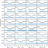 |
Fig. 4 Light curves of three full transits of WASP-74 b observed with MuSCAT2, a transit observed with GROND, seven transits observed with DK, two transits observed with CA, and two transits observed with Spitzer. A transit model in black corresponding to the median of the model parameter posteriors is shown. |
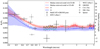 |
Fig. 5 Radius ratios in various passbands, including MuSCAT2 and GROND joint measurements (circles), GROND near-infrared observations (squares; Mancini et al. 2019), Calar Alto 1.23 m and Danish 1.54 m (triangles; Mancini et al. 2019), HST/WFC3 observations (no symbol) from Tsiaras et al. (2018), and Spitzer measurements (diamonds). The blue line shows the median retrieved atmospheric model based on all measurements and the light blue band its 1σ uncertainty. The red line and its shaded band show the retrieval without the measurements in the Cousins-I and Bessell-I bands. The small diamonds in cyan and yellow show the binned version of the retrieved model in the passbands with observations. HST/WFC3 measurements were shifted using the best-fit values from the two retrieval runs. |
Best-fit parameters from the atmospheric retrieval.
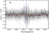 |
Fig. 6 Transmission spectrum of WASP-74 b in the Hα line, combining the three nights observed with the HARPS-N spectrograph. The original result is shown in light grey. The black dots correspond to the data binned by 0.1 Å. The error bars come from the propagated photon noise. |
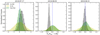 |
Fig. 7 Distributions of the EMC analysis in the Hα line, using 20 000 iterations and measuring the absorption depth with a bandwidth of 0.75 Å. Each panel corresponds to the analysis of one night. In green we present the “out-out” scenario, in yellow the “in-in”, and in grey the “in-out”, which corresponds to the atmospheric absorption scenario. The blue dashed vertical line indicates the zero absorption level. |
5.3 High-resolution transmission spectroscopy
High-resolution transmission spectroscopy observations are an excellent tool to study the atmospheric composition of exoplanets orbiting bright host stars (Wyttenbach et al. 2015, 2017; Seidel et al. 2019; Cauley et al. 2019). The one-dimensional HARPS-N spectra were corrected of the Earth telluric absorption contamination using Molecfit (Smette et al. 2015; Kausch et al. 2015), as described in Allart et al. (2017) and as adopted in recent atmospheric studies such as Hoeijmakers et al. (2018, 2019), Casasayas-Barris et al. (2019). After this correction, we followed the standard method to extract the atmospherictransmission spectrum (see e.g. Wyttenbach et al. 2015; Casasayas-Barris et al. 2018; Yan & Henning 2018; Yan et al. 2019, for details).
In particular, to move the spectra to the stellar rest frame, we used the stellar velocity semi-amplitude (K⋆ = 114.1 m s−1) measuredby Hellier et al. (2015). The master out-of-transit spectrum was computed by combining the out-of-transit data using the S/N of the order as weight. After computing the ratio of the spectra by this master out-of-transit spectrum, the residuals are moved to the planet rest frame using a planet velocity semi-amplitude Kp = 178.92 km s−1, derived from K⋆, and the planetary and stellar masses measured in this work (see Table 2). Finally, because of the long ingress and egress duration of the transit, only around four spectra were taken between the second and third contacts. For this reason, when computing the transmission spectrum, we averaged the spectra between the first and fourth contacts of the transit. We note that the selectionof the in- and out-of-transit observations was performed using the transit epoch measured in Sect. 4.
We applied this method to multiple lines of the spectrum. In the case of Na I, the S/N in the stellar lines core is too low to retrieve any atmospheric signature. For the first night, for example, the central core is at null counts level. Focussing on Hα (6562.81 Å; Kramida et al. 2019), we combined the results of the three transit observations by using the mean S/N of each night in Hα order as weights. The transmission spectrum is presented in Fig. 6. The results from the individual nights are presented inthe Appendix for completeness (Fig. A.1).
We also modelled the centre-to-limb variation (CLV) and RM effects in order to estimate the impact of both effects. For the CLV estimation, we followed Yan et al. (2017) and also included the RM effect on the stellar lines profile as presented in Yan & Henning (2018) and Casasayas-Barris et al. (2019). For this computation, the stellar spectra are modelled using VALD3 line list (Ryabchikova et al. 2015) and MARCS (Gustafsson et al. 2008) models, assuming solar abundance, local thermodynamic equilibrium, and the stellar parameters presented in Sect. 3. For the WASP-74 system these effects have an impact smaller than ~ 0.1% (in relative flux) in the Hα line core, which is included in error bars of the resulting transmission spectrum (see Fig. 6).
Thus, we are not able to detect any feature with atmospheric origin. The achieved S/N of the spectra is very low at the line cores, especially for deeper lines such as Na I. For this reason, and owing to the equilibrium temperature of the planet (1860 K), which is close to the UHJ zone, our study is focussed on the Hα line. The transmission spectrum around this spectral line does not show any clear signature from the exoplanet atmosphere. In order to account for possible systematic effects, we computed the empirical Monte Carlo analysis described in Redfield et al. (2008). Figure 7 shows that the “in-in” and “out-out” distributions are centred at zero absorption depth for all nights, as expected. On the other hand, the “in-out” distribution, which corresponds to the absorption scenario, is centred at a different position depending on the night. For the first and last nights, the absorption scenario cannot be disentangled from the noise level owing to the S/N achieved during the observations. However, for the second night where the S/N is the highest, the "in-out" distribution is centred at approximately − 0.3%. We note that with a transit duration of 2.38 h and using 600 s of integration per exposure, we are only able to measure around five spectra fully in-transit with relatively low S/N. The magnitude of the host star and its transit duration make WASP-74 b a challenging planet for atmospheric studies using 3.5 m telescopes. However, it is an ideal target to be studied using high-resolution spectrographs located on larger telescopes, such as ESPRESSO at the Very Large Telescope in Chile.
6 Summary
The obliquity of the WASP-74 system is measured for the first time, using three transits observed with the HARPS-N spectrograph. In this work, we measure an aligned system with a projected spin-orbit angle of 0.8 ± 1.0 degrees, in agreement with previous findings suggesting that planets orbiting stars with effective temperatures lower than ~ 6200 K are aligned.
We further use multi-colour observations of WASP-74 b to construct a transmission spectrum in order to probe its atmosphere. Our results disagree with those from Mancini et al. (2019), as we find no evidence of higher absorption in the bluer wavelengths, but a steep slope in the optical transmission spectrum. The origin of this disagreement is attributed to the different analyses of the light curves in the studies. We used the PLATON code to retrieve the atmospheric properties of WASP-74 b. We fit the combined transmission spectrum, including the low-resolution HST/WFC3 spectrum from Tsiaras et al. (2018), the GROND measurements and our new MuSCAT2 data. The retrieved transmission spectrum is almost featureless, except for the significant scattering slope in the optical.
Finally, using three transit observations of WASP-74 b with the HARPS-N spectrograph, we investigate its high-resolution transmission spectrum. Unfortunately, owing to the low S/N of the data, we are not able to detect any feature with atmospheric origin. The magnitude of the host star and its transit duration make WASP-74 b a challenging planet for atmospheric studies using 4 m class telescopes, but it is an interesting target to be further studied using high-resolution spectrographs placed in larger aperture telescopes.
Acknowledgements
This article is partly based on observations made with the MuSCAT2 instrument, developed by ABC, at Telescopio Carlos Sánchez operated on the island of Tenerife by the IAC in the Spanish Observatorio del Teide. It is also based on observations made with the Italian Telescopio Nazionale Galileo (TNG) operated on the island of La Palma by the Fundación Galileo Galilei of the INAF (Istituto Nazionale di Astrofisica) at the Spanish Observatorio del Roque de los Muchachos of the Instituto de Astrofisica de Canarias. R.L. has received funding from the European Union’s Horizon 2020 research and innovation program under the Marie Skłodowska-Curie grant agreement No. 713673 and financial support through the “la Caixa” INPhINIT Fellowship Grant LCF/BQ/IN17/11620033 for Doctoral studies at Spanish Research Centres of Excellence from “la Caixa” Banking Foundation, Barcelona, Spain. G.C. acknowledges the support by the B-type Strategic Priority Program of the Chinese Academy of Sciences (Grant No. XDB41000000) and the Natural Science Foundation of Jiangsu Province (Grant No. BK20190110). This work is partly financed by the Spanish Ministry of Economics and Competitiveness through grants ESP2013-48391-C4-2-R. This work is supported by JSPS KAKENHI grant Nos. 18H05442, 15H02063, 22000005, JP17H04574, JP18H01265, and JP18H05439, and JST PRESTO Grant Number JPMJPR1775.
Appendix A High-resolution transmission spectroscopy. Additional results
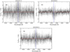 |
Fig. A.1 Individual transmission spectra around Hα line. The original data are shown in light grey, while in black dots the data are binned by 0.1 Å. In The Hα laboratory position is shown in blue and the null absorption level is indicated in red. |
References
- Addison, B. C., Wang, S., Johnson, M. C., et al. 2018, AJ, 156, 197 [NASA ADS] [CrossRef] [Google Scholar]
- Albrecht, S., Winn, J. N., Johnson, J. A., et al. 2012, ApJ, 757, 18 [NASA ADS] [CrossRef] [Google Scholar]
- Allart, R., Lovis, C., Pino, L., et al. 2017, A&A, 606, A144 [NASA ADS] [CrossRef] [EDP Sciences] [Google Scholar]
- Beichman, C., Livingston, J., Werner, M., et al. 2016, ApJ, 822, 39 [NASA ADS] [CrossRef] [Google Scholar]
- Bourrier, V., Cegla, H. M., Lovis, C., & Wyttenbach, A. 2017, A&A, 599, A33 [NASA ADS] [CrossRef] [EDP Sciences] [Google Scholar]
- Brahm, R., Jordán, A., Hartman, J., & Bakos, G. 2017, MNRAS, 467, 971 [NASA ADS] [Google Scholar]
- Bressan, A., Marigo, P., Girardi, L., et al. 2012, MNRAS, 427, 127 [NASA ADS] [CrossRef] [Google Scholar]
- Casasayas-Barris, N., Palle, E., Nowak, G., et al. 2017, A&A, 608, A135 [NASA ADS] [CrossRef] [EDP Sciences] [Google Scholar]
- Casasayas-Barris, N., Pallé, E., Yan, F., et al. 2018, A&A, 616, A151 [NASA ADS] [CrossRef] [EDP Sciences] [Google Scholar]
- Casasayas-Barris, N., Pallé, E., Yan, F., et al. 2019, A&A, 628, A9 [NASA ADS] [CrossRef] [EDP Sciences] [Google Scholar]
- Cauley, P. W., Shkolnik, E. L., Ilyin, I., et al. 2019, AJ, 157, 69 [NASA ADS] [CrossRef] [Google Scholar]
- Cegla, H. M., Lovis, C., Bourrier, V., et al. 2016, A&A, 588, A127 [NASA ADS] [CrossRef] [EDP Sciences] [Google Scholar]
- Cosentino, R., Lovis, C., Pepe, F., et al. 2014, SPIE Conf. Ser., 9147, 91478C [Google Scholar]
- Cosentino, R., Lovis, C., Pepe, F., et al. 2012, Proc. SPIE, 8446, 84461V [Google Scholar]
- Czesla, S., Schröter, S., Schneider, C. P., et al. 2019, PyA: Python astronomy-related packages [Google Scholar]
- Deming, D., Knutson, H., Kammer, J., et al. 2015, ApJ, 805, 132 [NASA ADS] [CrossRef] [Google Scholar]
- Dragomir, D., Benneke, B., Pearson, K. A., et al. 2015, ApJ, 814, 102 [NASA ADS] [CrossRef] [Google Scholar]
- Ehrenreich, D., Bonfils, X., Lovis, C., et al. 2014, A&A, 570, A89 [NASA ADS] [CrossRef] [EDP Sciences] [Google Scholar]
- Espinoza, N., Rackham, B. V., Jordán, A., et al. 2019, MNRAS, 482, 2065 [Google Scholar]
- Evans, T. M., Sing, D. K., Wakeford, H. R., et al. 2016, ApJ, 822, L4 [NASA ADS] [CrossRef] [Google Scholar]
- Evans, T. M., Sing, D. K., Kataria, T., et al. 2017, Nature, 548, 58 [NASA ADS] [CrossRef] [Google Scholar]
- Evans, T. M., Sing, D. K., Goyal, J. M., et al. 2018, AJ, 156, 283 [NASA ADS] [CrossRef] [Google Scholar]
- Foreman-Mackey, D., Hogg, D. W., Lang, D., & Goodman, J. 2013, PASP, 125, 306 [CrossRef] [Google Scholar]
- Fortney, J. J., Lodders, K., Marley, M. S., & Freedman, R. S. 2008, ApJ, 678, 1419 [NASA ADS] [CrossRef] [Google Scholar]
- Gaia Collaboration (Brown, A. G. A., et al.) 2018, A&A, 616, A1 [NASA ADS] [CrossRef] [EDP Sciences] [Google Scholar]
- GAPS Collaboration (Smareglia, R., et al.) 2014, ASP Conf. Ser., 485, 435 [NASA ADS] [Google Scholar]
- Garhart, E., Deming, D., Mandell, A., et al. 2020, AJ, 159, 137 [NASA ADS] [CrossRef] [Google Scholar]
- Gustafsson, B., Edvardsson, B., Eriksson, K., et al. 2008, A&A, 486, 951 [NASA ADS] [CrossRef] [EDP Sciences] [Google Scholar]
- Haynes, K., Mandell, A. M., Madhusudhan, N., Deming, D., & Knutson, H. 2015, ApJ, 806, 146 [NASA ADS] [CrossRef] [Google Scholar]
- Hébrard, G., Ehrenreich, D., Bouchy, F., et al. 2011, A&A, 527, L11 [NASA ADS] [CrossRef] [EDP Sciences] [Google Scholar]
- Hellier, C., Anderson, D. R., Collier Cameron, A., et al. 2015, AJ, 150, 18 [NASA ADS] [CrossRef] [Google Scholar]
- Hoeijmakers, H. J., Ehrenreich, D., Heng, K., et al. 2018, Nature, 560, 453 [NASA ADS] [CrossRef] [Google Scholar]
- Hoeijmakers, H. J., Ehrenreich, D., Kitzmann, D., et al. 2019, A&A, 627, A165 [NASA ADS] [CrossRef] [EDP Sciences] [Google Scholar]
- Høg, E., Fabricius, C., Makarov, V. V., et al. 2000, A&A, 355, L27 [Google Scholar]
- Hubeny, I., Burrows, A., & Sudarsky, D. 2003, ApJ, 594, 1011 [NASA ADS] [CrossRef] [Google Scholar]
- Kausch, W., Noll, S., Smette, A., et al. 2015, A&A, 576, A78 [NASA ADS] [CrossRef] [EDP Sciences] [Google Scholar]
- Kawashima, Y., & Ikoma, M. 2019, ApJ, 877, 109 [CrossRef] [Google Scholar]
- Knutson, H. A., Howard, A. W., & Isaacson, H. 2010, ApJ, 720, 1569 [NASA ADS] [CrossRef] [Google Scholar]
- Knutson, H. A., Lewis, N., Fortney, J. J., et al. 2012, ApJ, 754, 22 [NASA ADS] [CrossRef] [Google Scholar]
- Kramida, A., Yu. Ralchenko, Reader, J., & NIST ASD Team. 2019, NIST Atomic Spectra Database (ver. 5.5.2), Available at https://physics.nist.gov/asd [2019, September 15]. National Institute of Standards and Technology, Gaithersburg, MD. [Google Scholar]
- Livingston, J. H., Crossfield, I. J. M., Werner, M. W., et al. 2019, AJ, 157, 102 [NASA ADS] [CrossRef] [Google Scholar]
- Madhusudhan, N. 2012, ApJ, 758, 36 [NASA ADS] [CrossRef] [Google Scholar]
- Mancini, L., Southworth, J., Mollière, P., et al. 2019, MNRAS, 485, 5168 [NASA ADS] [CrossRef] [Google Scholar]
- Mayor, M., Pepe, F., Queloz, D., et al. 2003, The Messenger, 114, 20 [NASA ADS] [Google Scholar]
- McLaughlin, D. B. 1924, ApJ, 60, 22 [NASA ADS] [CrossRef] [Google Scholar]
- Narita, N., Fukui, A., Kusakabe, N., et al. 2019, J. Astron. Telesc. Instrum. Syst., 5, 015001 [NASA ADS] [Google Scholar]
- Nugroho, S. K., Kawahara, H., Masuda, K., et al. 2017, AJ, 154, 221 [NASA ADS] [CrossRef] [Google Scholar]
- Ohno, K., & Kawashima, Y. 2020, ApJ, 895, L47 [CrossRef] [Google Scholar]
- Ormel, C. W., & Min, M. 2019, A&A, 622, A121 [NASA ADS] [CrossRef] [EDP Sciences] [Google Scholar]
- Oshagh, M., Santos, N. C., Ehrenreich, D., et al. 2014, A&A, 568, A99 [NASA ADS] [CrossRef] [EDP Sciences] [Google Scholar]
- Oshagh, M., Triaud, A. H. M. J., Burdanov, A., et al. 2018, A&A, 619, A150 [NASA ADS] [CrossRef] [EDP Sciences] [Google Scholar]
- Parmentier, V., Line, M. R., Bean, J. L., et al. 2018, A&A, 617, A110 [NASA ADS] [CrossRef] [EDP Sciences] [Google Scholar]
- Parviainen, H. 2015, MNRAS, 450, 3233 [NASA ADS] [CrossRef] [Google Scholar]
- Parviainen, H. 2018, Handbook of Exoplanets (Berlin: Springer), 149 [Google Scholar]
- Parviainen, H., & Aigrain, S. 2015, MNRAS, 453, 3821 [Google Scholar]
- Parviainen, H., Tingley, B., Deeg, H. J., et al. 2019, A&A, 630, A89 [NASA ADS] [CrossRef] [EDP Sciences] [Google Scholar]
- Pino, L., Désert, J.-M., Brogi, M., et al. 2020, ApJ, 894, L27 [Google Scholar]
- Pont, F., Zucker, S., & Queloz, D. 2006, MNRAS, 373, 231 [NASA ADS] [CrossRef] [Google Scholar]
- Rackham, B. V., Apai, D., & Giampapa, M. S. 2018, ApJ, 853, 122 [Google Scholar]
- Rackham, B. V., Apai, D., & Giampapa, M. S. 2019, AJ, 157, 96 [NASA ADS] [CrossRef] [Google Scholar]
- Redfield, S., Endl, M., Cochran, W. D., & Koesterke, L. 2008, ApJ, 673, L87 [NASA ADS] [CrossRef] [MathSciNet] [Google Scholar]
- Rossiter, R. A. 1924, ApJ, 60, 15 [Google Scholar]
- Ryabchikova, T., Piskunov, N., Kurucz, R. L., et al. 2015, Phys. Scr., 90, 054005 [Google Scholar]
- Sedaghati, E., Boffin, H. M. J., MacDonald, R. J., et al. 2017, Nature, 549, 238 [NASA ADS] [CrossRef] [Google Scholar]
- Seidel, J. V., Ehrenreich, D., Wyttenbach, A., et al. 2019, A&A, 623, A166 [NASA ADS] [CrossRef] [EDP Sciences] [Google Scholar]
- Sing, D. K., Wakeford, H. R., Showman, A. P., et al. 2015, MNRAS, 446, 2428 [NASA ADS] [CrossRef] [Google Scholar]
- Skrutskie, M. F., Cutri, R. M., Stiening, R., et al. 2006, AJ, 131, 1163 [NASA ADS] [CrossRef] [Google Scholar]
- Smette, A., Sana, H., Noll, S., et al. 2015, A&A, 576, A77 [NASA ADS] [CrossRef] [EDP Sciences] [Google Scholar]
- Southworth, J. 2011, MNRAS, 417, 2166 [NASA ADS] [CrossRef] [Google Scholar]
- Spiegel, D. S., Silverio, K., & Burrows, A. 2009, ApJ, 699, 1487 [NASA ADS] [CrossRef] [Google Scholar]
- Triaud, A. H. M. J. 2017, Handbook of Exoplanets (Springer Living Reference Work) (Berlin: Springer), 2 [Google Scholar]
- Triaud, A. H. M. J., Collier Cameron, A., Queloz, D., et al. 2010, A&A, 524, A25 [NASA ADS] [CrossRef] [EDP Sciences] [Google Scholar]
- Tsiaras, A., Waldmann, I. P., Zingales, T., et al. 2018, AJ, 155, 156 [NASA ADS] [CrossRef] [Google Scholar]
- Wakeford, H. R., & Sing, D. K. 2015, A&A, 573, A122 [NASA ADS] [CrossRef] [EDP Sciences] [Google Scholar]
- Winn, J. N. 2010, Exoplanet Transits and Occultations (Tucson, AZ: University of Arizona Press), 55 [Google Scholar]
- Winn, J. N., Fabrycky, D., Albrecht, S., & Johnson, J. A. 2010, ApJ, 718, L145 [NASA ADS] [CrossRef] [Google Scholar]
- Winn, J. N., Holman, M. J., Torres, G., et al. 2008, ApJ, 683, 1076 [NASA ADS] [CrossRef] [Google Scholar]
- Winn, J. N., Noyes, R. W., Holman, M. J., et al. 2005, ApJ, 631, 1215 [NASA ADS] [CrossRef] [Google Scholar]
- Wyttenbach, A., Ehrenreich, D., Lovis, C., Udry, S., & Pepe, F. 2015, A&A, 577, A62 [NASA ADS] [CrossRef] [EDP Sciences] [Google Scholar]
- Wyttenbach, A., Lovis, C., Ehrenreich, D., et al. 2017, A&A, 602, A36 [NASA ADS] [CrossRef] [EDP Sciences] [Google Scholar]
- Yan, F., & Henning, T. 2018, Nat. Astron., 2, 714 [NASA ADS] [CrossRef] [Google Scholar]
- Yan, F., Pallé, E., Fosbury, R. A. E., Petr-Gotzens, M. G., & Henning, T. 2017, A&A, 603, A73 [NASA ADS] [CrossRef] [EDP Sciences] [Google Scholar]
- Yan, F., Casasayas-Barris, N., Molaverdikhani, K., et al. 2019, A&A 632, A69 [NASA ADS] [CrossRef] [EDP Sciences] [Google Scholar]
- Yan, F., Pallé, E., Reiners, A., et al. 2020, A&A, 640, L5 [CrossRef] [EDP Sciences] [Google Scholar]
- Zechmeister, M., Reiners, A., Amado, P. J., et al. 2018, A&A, 609, A12 [CrossRef] [Google Scholar]
- Zhang, M., Chachan, Y., Kempton, E. M. R., & Knutson, H. A. 2019, PASP, 131, 034501 [NASA ADS] [CrossRef] [Google Scholar]
All Tables
Stellar and planetary parameters derived from the multi-colour joint transit analysis of WASP-74 b.
All Figures
|
Fig. 1 Stellar RVs of WASP-74 for each individual night. The RV measurements are shown in black dots. The best-fit model obtained with the MCMC procedure is shown in cyan. |
| In the text | |
|
Fig. 2 Rossiter-McLaughlin effect during the transit of WASP-74 b after being detrended (top panel), and residuals between the data and model (bottom panel). The RVs from the three different data sets are shown with different symbols. The dark blue line corresponds to the best-fit RM model. The 1σ and 3σ uncertainties of the model are indicated in light blue. |
| In the text | |
|
Fig. 3 Measurements of orbital obliquity for the known transiting extrasolar planetary systems and brown dwarf companions in front of the effective temperature of the host star (dots), extracted from TEPCat orbital obliquity catalogue (Southworth 2011). The planetary radius is presented in the colour bar. The star symbol corresponds to the spin-orbit measurement of WASP-74 b. The black-dashed vertical line denotes the 6250 K effective temperature transition from Winn et al. (2010). |
| In the text | |
|
Fig. 4 Light curves of three full transits of WASP-74 b observed with MuSCAT2, a transit observed with GROND, seven transits observed with DK, two transits observed with CA, and two transits observed with Spitzer. A transit model in black corresponding to the median of the model parameter posteriors is shown. |
| In the text | |
|
Fig. 5 Radius ratios in various passbands, including MuSCAT2 and GROND joint measurements (circles), GROND near-infrared observations (squares; Mancini et al. 2019), Calar Alto 1.23 m and Danish 1.54 m (triangles; Mancini et al. 2019), HST/WFC3 observations (no symbol) from Tsiaras et al. (2018), and Spitzer measurements (diamonds). The blue line shows the median retrieved atmospheric model based on all measurements and the light blue band its 1σ uncertainty. The red line and its shaded band show the retrieval without the measurements in the Cousins-I and Bessell-I bands. The small diamonds in cyan and yellow show the binned version of the retrieved model in the passbands with observations. HST/WFC3 measurements were shifted using the best-fit values from the two retrieval runs. |
| In the text | |
|
Fig. 6 Transmission spectrum of WASP-74 b in the Hα line, combining the three nights observed with the HARPS-N spectrograph. The original result is shown in light grey. The black dots correspond to the data binned by 0.1 Å. The error bars come from the propagated photon noise. |
| In the text | |
|
Fig. 7 Distributions of the EMC analysis in the Hα line, using 20 000 iterations and measuring the absorption depth with a bandwidth of 0.75 Å. Each panel corresponds to the analysis of one night. In green we present the “out-out” scenario, in yellow the “in-in”, and in grey the “in-out”, which corresponds to the atmospheric absorption scenario. The blue dashed vertical line indicates the zero absorption level. |
| In the text | |
|
Fig. A.1 Individual transmission spectra around Hα line. The original data are shown in light grey, while in black dots the data are binned by 0.1 Å. In The Hα laboratory position is shown in blue and the null absorption level is indicated in red. |
| In the text | |
Current usage metrics show cumulative count of Article Views (full-text article views including HTML views, PDF and ePub downloads, according to the available data) and Abstracts Views on Vision4Press platform.
Data correspond to usage on the plateform after 2015. The current usage metrics is available 48-96 hours after online publication and is updated daily on week days.
Initial download of the metrics may take a while.