| Issue |
A&A
Volume 642, October 2020
|
|
|---|---|---|
| Article Number | A111 | |
| Number of page(s) | 13 | |
| Section | Galactic structure, stellar clusters and populations | |
| DOI | https://doi.org/10.1051/0004-6361/202037641 | |
| Published online | 12 October 2020 | |
A study on tidal disruption event dynamics around an Sgr A*-like massive black hole
Center for Astrophysics and Cosmology, University of Nova Gorica, Vipavska 11c, 5270 Ajdovščina, Slovenia
e-mail: This email address is being protected from spambots. You need JavaScript enabled to view it.
Received:
2
February
2020
Accepted:
14
July
2020
Abstract
Context. The number of observed tidal disruption events is increasing rapidly with the advent of new surveys. Thus, it is becoming increasingly important to improve tidal disruption event models using different stellar and orbital parameters.
Aims. We study the dynamical behaviour of tidal disruption events produced by an Sgr A*-like massive black hole by changing different initial orbital parameters, taking into account the observed orbits of S stars. Investigating different types of orbits and penetration factors is important since their variations lead to different timescales of the tidal disruption event debris dynamics, making mechanisms such as self-crossing and pancaking act strongly or weakly and thus affecting the circularisation and accretion disc formation.
Methods. We performed smoothed particle hydrodynamics simulations. Each simulation consisted of modelling the star with 105 particles, and the density profile is described by a polytrope with γ = 5/3. The massive black hole was modelled with a generalised post-Newtonian potential, which takes into account the relativistic effects of the Schwarzschild space-time.
Results. Our analyses find that mass return rate distributions of solar-like stars and S-like stars with the same eccentricities have similar durations, but S-like stars have higher mass return rate distributions, as expected due to their larger masses. Regarding debris circularisation, we identify four types of evolution related to the mechanisms and processes involved during circularisation: in type 1, the debris does not circularise efficiently, hence a disc is not formed or is formed after a relatively long time; in type 2, the debris slowly circularises and eventually forms a disc with no debris falling back; in type 3, the debris circularises relatively quickly and forms a disc while there is still debris falling back; in type 4, the debris quickly and efficiently circularises, mainly through self-crossings and shocks, and forms a disc with no debris falling back. Finally, we find that the standard relation of circularisation radius rcirc = 2rt holds only for β = 1 and eccentricities close to parabolic.
Key words: hydrodynamics / methods: numerical / black hole physics / Galaxy: nucleus / accretion, accretion disks
© ESO 2020
1. Introduction
It is well established from both gas and stellar dynamical measurements that massive black holes (MBHs) reside in the nuclei of most galaxies (e.g. Magorrian & Tremaine 1999, and references therein). These extreme astrophysical objects have masses between 105 M⊙ and 1010 M⊙ and are embedded in dense stellar environments, as can be observed from the nearest MBH we can study, that is to say Sgr A* in our Galactic centre (GC). While nearby MBHs can be studied dynamically, distant ones can only be observed if they are undergoing luminous accretion. This is the case for active galactic nuclei (AGNs), which provide the most valuable information about MBHs; however, they represent a small fraction of the MBH population. In order to form a more complete picture of the astrophysical properties of MBHs, it is necessary to also probe those that are in a quiescent state.
A variety of dynamical processes are capable of feeding stars into MBHs; this can result in tidal disruption events (TDEs), which can temporarily turn on a dormant MBH. Amongst these feeding mechanisms, the two-body relaxation is the most understood. Calculations of TDE rates based on this mechanism in realistic galaxies find that they are rare events, with a rate of ≳10−4 yr−1 (Wang & Merritt 2004; Stone & Metzger 2016; Stone & van Velzen 2016). In comparison, observational estimates for the TDE rate are typically ∼10−5 yr−1 (Donley et al. 2002; Khabibullin & Sazonov 2014), which is discrepant by an order of magnitude (or more) with theoretical estimates (Stone & Metzger 2016). Other processes can, in principle, enhance the TDE rate above the order set by two-body relaxation, such as: the non-conservation of angular momentum in axisymmetric or triaxial potentials (Magorrian & Tremaine 1999; Merritt & Poon 2004); interactions with massive perturbers (Mp > 102 M⊙), such as molecular clouds, globular stellar clusters, intermediate MBHs (Perets et al. 2007), and large-scale accretion discs (Karas & Šubr 2007); and gravitational wave recoil of the central MBH (Stone & Loeb 2011). The impact of these more exotic mechanisms is harder to quantify observationally.
The general picture of a TDE (Lacy et al. 1982; Carter & Luminet 1983; Rees 1988; Phinney 1989; Evans & Kochanek 1989) considers a star approaching an MBH on a nearly parabolic orbit from large separation (∼pc). After the star gets squeezed and disrupted by the MBH, approximately half of the stellar debris loses orbital energy inside the tidal disruption radius and becomes gravitationally bound to the MBH. The bound debris falls back, circularises due to self-crossings and collisional shocks between gas streams, and eventually accretes into the MBH. The properties of this accretion disc have been investigated by many authors (e.g. Cannizzo et al. 1990; Loeb & Ulmer 1997; Strubbe & Quataert 2009; Lodato & Rossi 2011; Shen & Matzner 2014). The power emitted during the accretion process is enough to generate a highly luminous event; several of these events have been observed (Bade et al. 1996; Komossa et al. 1999; Halpern et al. 2004; Bloom et al. 2011; Cenko et al. 2012; Bogdanović et al. 2014; Komossa 2015). The catalogue of TDE candidates is steadily growing as more of them are detected at optical, ultraviolet, and soft X-ray wavelengths (e.g. Bade et al. 1996; Komossa & Greiner 1999; Gezari et al. 2006); thanks to high-cadence surveys, a larger fraction of these observed events have well-sampled lightcurves that include the early rise to peak (e.g. Gezari et al. 2012; Arcavi et al. 2014; Chornock et al. 2014; Blagorodnova et al. 2019). A few of them are thought to produce a relativistic jet launched from the inner region of the accretion flow, to which the observed hard X-ray emission is attributed (Bloom et al. 2011; Cenko et al. 2012; Brown et al. 2015).
It has been analytically shown (Rees 1988; Phinney 1989) that the rate at which debris returns to the MBH is dm/dt ∝ t−5/3. This feature is considered to be the observational signature of a TDE. Indeed, many of the observed TDE candidates show a lightcurve that follows this power-law. However, this feature is expected for the bolometric lightcurve and for the X-ray band, while the optical and ultraviolet bands are expected to follow a flatter dependence ∝t−5/12 (Lodato & Rossi 2011). Observationally, on one hand TDEs are found to follow the t−5/3 feature in the first few months (e.g. Gezari et al. 2008); on the other hand, there are TDEs that are best approximated by the t−5/12 (Holoien et al. 2019). Furthermore, TDEs such as ASASSN-14li and ASASSN-14ae are found to be best fitted with an exponential law e−t (e.g. Holoien et al. 2014, 2016).
The dynamics of stellar tidal disruption has been modelled by several authors, starting with simple analytical considerations (Rees 1988; Phinney 1989; Lodato et al. 2009; Kesden 2012), going to more complex dynamical models (e.g. Luminet & Marck 1985; Kosovichev & Novikov 1992; Ivanov & Novikov 2001; Gomboc & Čadež 2005) and hydrodynamical simulations (e.g. Nolthenius & Katz 1982; Evans & Kochanek 1989; Laguna et al. 1993; Kobayashi et al. 2004; Guillochon et al. 2009; Rosswog et al. 2009; Antonini et al. 2011; Shiokawa et al. 2015; Bonnerot & Lu 2020). As the number of observed TDEs increases, it becomes more important to improve models of dm/dt for disruptions with different stellar and orbital parameters. Early smoothed particle hydrodynamics (SPH) calculations (Evans & Kochanek 1989) supported the initial analytic estimates, showing that the distribution of specific energies, calculated not long after the time of disruption, produces a fallback rate ∝t−5/3. Lodato et al. (2009) investigated the effects of the structure of the star on the disruption process and demonstrated that the early stages of the fallback depend on the properties of the star. Guillochon & Ramirez-Ruiz (2013) find that shallower impact parameters affect the nature of the event, often resulting in the survival of a bound stellar core (partial disruption). Dai et al. (2013), Hayasaki et al. (2013, 2016), Bonnerot et al. (2016), Shiokawa et al. (2015), and Liptai et al. (2019) studied stars on elliptical orbits and the effects of general relativity on the stream and show how apsidal and Lense-Thirring precession can alter the formation of the disc that forms when the tidally disrupted debris returns to pericentre.
The GC is a unique laboratory to study physical processes and phenomena that may be occurring in many other galactic nuclei, where they are not observationally accessible. The general picture of the GC, in particular that of the central parsecs, is rapidly changing (e.g. Yusef-Zadeh et al. 2000; Alexander 2005; Yusef-Zadeh & Wardle 2012). In order to understand the stellar environment in the inner parsecs, it is relevant to study the stars well outside the dynamical sphere of influence of Sgr A* and within the ≤100 pc scale. The Galactic bulge stellar population is composed of old stars (∼10 Gyr), while the inner ≤100 pc stellar population seems to have been formed throughout the life of the Galaxy. In particular, the discovery of the so-called “S stars”, which orbit Sgr A* (< 0.04 pc), has provided a new way to study Sgr A*. However, their great proximity to the MBH was soon called the “paradox of youth” (Ghez et al. 2003). The S stars that have been analysed are young, main sequence massive stars, and their existence was unexpected as it is not clear how they could form in such a violent environment. A current idea is that these stars formed far from the central region, to which they migrated through the Hills mechanism (Hills 1988; Brown 2015). In this scenario, we start with binary stars, which get scattered under certain dynamical conditions towards the MBH. Due to the interaction with the MBH, one of the binary components gets ejected at high velocity (high velocity star), while the other gets on a bound orbit to the MBH. There is an interesting mechanism outlined by Hamers & Perets (2017), which involves nuclear spiral arms in the enhancement of TDEs, S stars, and high velocity stars’ rates. On the ∼100 pc scale, gas can be perturbed by torques from nuclear bars (e.g. Shlosman et al. 1989; Englmaier & Shlosman 2004), which drive inflows to the nuclear regions, giving rise to nuclear spiral arms. These structures are an additional channel that can drive stars onto disruption orbits with the MBH.
To better characterise TDEs, in this paper we study the TDE dynamical behaviour through different initial orbital parameters of a star, considering the stellar environment offered in the GC. This paper is organised as follows: in Sect. 2, a description of the simulations setup is given; in Sect. 3, we present results of simulations, focusing on specific energy and mass return rate distributions and on circularisation mechanisms; in Sect. 4 we give our conclusions.
2. SPH simulations
2.1. Method
We performed SPH simulations with the fast, modular, and low-memory Phantom1 code (Price et al. 2018). Smoothed particle hydrodynamics is a particle technique (Gingold & Monaghan 1977; Lucy 1977) (see e.g. Monaghan 1992, for a review) that divides a fluid into a set of discrete fluid elements (i.e. the particles), whose physical quantities are computed with a smoothing kernel. The Phantom code is used to solve different astrophysical problems, and it has been successfully employed to study TDEs (e.g. Coughlin & Nixon 2015; Coughlin et al. 2016a,b; Bonnerot et al. 2016; Golightly et al. 2019a).
The simulations were performed in two stages: first, the desired star was modelled as a polytropic gas sphere; then, the tidal disruption process was performed. The star was modelled as a polytrope with index γ = 5/3, as it well approximates the density distribution of main sequence stars. The polytropic profile was achieved by arranging ∼105 particles on a closed-packed sphere configuration, which was stretched to get the desired density distribution. This initial gas sphere was allowed to collapse under self-gravity using the polytropic equation of state P = Kρ1 + 1/n, where K is a constant and n is the polytropic index. In addition, the star so formed was relaxed in isolation to smooth out numerically induced perturbations. Finally, the star was placed on the desired trajectory to disruption.
The gas evolves according to the gravity of the MBH, which is modelled with the gravitational potential given by Tejeda & Rosswog (2013):
![Mathematical equation: $$ \begin{aligned}&\Phi _G(r,\dot{r},\dot{\phi }) = -\frac{GM_{\rm BH}}{r} - \left(\frac{2r_{\rm g}}{r-2r_{\rm g}}\right)\nonumber \\&\quad \qquad \qquad \left[\left(\frac{r-r_{\rm g}}{r-2r_{\rm g}}\right)\dot{r}^2\! +\! \frac{r^2(\dot{\theta }^2+\sin ^2\theta \dot{\phi }^2)}{2}\right] , \end{aligned} $$](/articles/aa/full_html/2020/10/aa37641-20/aa37641-20-eq1.gif) (1)
(1)
where rg = GMBH/c2 is the gravitational radius, θ is the polar angle, and ϕ is the azimuthal angle in spherical geometry. This potential accurately models several relativistic features of the Schwarzschild space-time, reproducing, in particular, the exact location of the marginally stable, marginally bound, and photon circular orbits, as well as the exact radial dependence of the binding energy and angular momentum. Moreover, this potential exactly reproduces the time evolution of parabolic-like trajectories and the pericentre advance of elliptical-like trajectories. A test particle evolving under this generalised Newtonian potential conserves the specific orbital energy and angular momentum given by
![Mathematical equation: $$ \begin{aligned} \epsilon = \frac{1}{2}\left[\frac{r^2\dot{r}^2}{(r-2r_{\rm g})^2} + \frac{r^3(\dot{\theta }^2+\sin ^2\theta \dot{\phi ^2})}{r-2r_{\rm g}}\right] - \frac{GM_{\rm BH}}{r} ,\end{aligned} $$](/articles/aa/full_html/2020/10/aa37641-20/aa37641-20-eq2.gif) (2)
(2)
 (3)
(3)
2.2. Stellar and orbital parameters
Since we wanted to study the dynamics of TDEs occurring in a nuclear environment like our GC, we chose an MBH and stars that are representative for such an environment. The mass of the MBH was, therefore, chosen to be the mass of Sgr A*, MBH = 4.3 M⊙ (Gillessen et al. 2009). We defined an accretion radius (i.e. a distance within which we remove any particle from the simulation due to accretion to the MBH), and we set this distance to be at the innermost stable circular orbit for a non-spinning black hole, rISCO = 6rg.
Most TDE simulations found in the literature study the disruption of solar type stars, that is stars with M* = M⊙ and R* = 1 R⊙ (e.g. Laguna et al. 1993; Ayal et al. 2000; Coughlin & Nixon 2015). For comparison purposes, we chose this kind of star for our simulations and, in addition, we chose a star with M* = 10 M⊙ and R* = 5 R⊙; this choice comes from the observation that the group of stars orbiting around Sgr A* within a distance of < 0.04 pc are S stars, which are massive main sequence stars. According to the recent study made by Habibi et al. (2017), high resolution spectroscopy infers that the spectral type of these stars is B0-B3V, that their masses range between 8–14 M⊙, that their radii range between 4–6 R⊙, and that their ages are < 15 Myr. It should be noted that we do not assume anything else about the stellar structure (discussion in Sect. 4).
In order to explore the stellar disruption evolution of the two chosen types of stars, we ran simulations for a range of orbital parameters. Considering that S stars have been observed to have eccentricities in the range of ∼0.4–0.95 (Eisenhauer et al. 2005; Parsa et al. 2017), we performed simulations for such orbits. We notice that below e = 0.5 our simulations do not show dynamically interesting TDEs for this study; therefore, we opted for 0.5 ≤ e ≤ 0.99. We added the high eccentricity e = 0.99 orbit to include stars scattered from large distances (on nearly parabolic orbits).
To study the effects of the strength of a tidal disruption, we chose different penetration factors β = rt/rp (where rt ≃ R*(MBH/M*)1/3 is the tidal radius, the distance at which a star can be disrupted by the MBH, and rp is the pericentre distance of the star’s centre of mass from the MBH). We chose orbits with β between 1 and 5. In order for a complete disruption to occur outside the MBH, the rp of the star’s orbit must be ≤rt, and rt must be greater than the MBH event horizon, 2rg. Panel a in Fig. 1 shows how orbits with fixed β change with eccentricities, and panel b shows how orbits with fixed e change with different β.
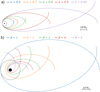 |
Fig. 1. Orbits with eccentricities ranging from e = 0.6 to 0.95 with fixed β = 1 (a), and orbits with penetration ranging from β = 1 to 5 with fixed e = 0.8 (b). Each orbit is the trajectory of the centre of mass of a star in the generalised Newtonian potential (Eq. (1)) in one period. The filled circle represents the rISCO, while the dashed circle represents the rt. |
The list of the 37 performed simulations is given in Table 1. Each simulation is labelled with the letter S or s, denoting an M* = 10 M⊙, R* = 5 R⊙ star (S star-like) and an M* = 1 M⊙, R* = 1 R⊙ star (solar-like), respectively, as well as a number denoting the β value and a number following a dot denoting the eccentricity.
Simulations.
Simulation data in this paper were visualised using the SPLASH tool (Price 2007). Figure 2 shows a sequence of snapshots of model S1.8.
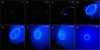 |
Fig. 2. Sequence of snapshots of model S1.8. The MBH is represented by the full white circle, which has a radius equal to rISCO, while the dashed white line represents the tidal radius rt. In panel a, the star is in its initial position ra and orbits the MBH on an anti-clockwise trajectory. In panel b, the star has been disrupted and the debris formed two tails, which will stretch and fall back (panel c). In panels d–g, the debris is going through circularisation processes, which result in the formation of a disc (panel h). |
3. Results and discussion
3.1. Specific energy and mass return rate distribution
Let us assume as an initial condition that the star at a large distance from the MBH is in hydrostatic equilibrium. We consider each fluid element of the star to initially move in a Keplerian orbit, each one with its own energy and thus each with an eccentricity close to that of the centre of mass of the star. As the star approaches the MBH, the orbits get squeezed, resulting in a perturbed hydrostatic equilibrium. The energy inside the star is redistributed, and the specific energy distribution will be wider, with a spread in energy (Stone et al. 2013)
 (4)
(4)
After the close approach to the MBH, the fluid elements move along orbits according to their new specific energy with a distribution ranging over
 (5)
(5)
where ϵorb is the specific orbital energy of the stellar centre of mass approaching the MBH. For eccentric orbits, ϵorb is given by
 (6)
(6)
Since we are interested in fluid elements that will form an accretion disc, we consider those with negative energies. These will return close to rp after a Keplerian period
 (7)
(7)
The most tightly bound debris and the most loosely bound debris have periods tmin and tmax, respectively, which can be calculated as (Hayasaki et al. 2013)
 (8)
(8)
![Mathematical equation: $$ \begin{aligned} t_{\rm max} = \frac{\pi }{\sqrt{2}}t_{\rm dyn}\left[\frac{\beta (1-e)}{2}\left(\frac{M_*}{M_{\rm BH}}\right)^{1/3}\right]^{-3/2} ,\end{aligned} $$](/articles/aa/full_html/2020/10/aa37641-20/aa37641-20-eq9.gif) (9)
(9)
where tdyn is the dynamical time given by  , and tmax is valid for e < ecrit, where ecrit ≈ 1−2/β(M*/MBH)1/3 is the eccentricity below which all the debris remains bound after disruption (amongst our models only S1.99 and s1.99 have e > ecrit). Thus, the duration time of mass fallback of eccentric TDEs with e < ecrit can be predicted to be finite and it is given by Δt = tmax − tmin. We calculated tmin and tmax analytically using Eqs. (8) and (9) and we find discrepancies with values obtained from our simulations. For example, Eqs. (8) and (9) give tmin = 0.002 yr and tmax = 0.005 yr for S1.6, and tmin = 0.001 yr and tmax = 0.003 yr for S3.8. The tmin values do not agree with values found from simulations (see Fig. 3, right-hand panels), where we find tmin ≈ 0.004 and tmax ≈ 0.005 for S1.6 and tmin ≈ 0.002 and tmax ≈ 0.003 for S3.8. This is due to the fact that they are evaluated taking into account the energy spread Δϵ, which is fixed by Eq. (4). This discrepancy has previously been noted by Hayasaki et al. (2013).
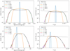 |
Fig. 3. Specific energy distribution (left) and corresponding fallback mass rates (right) of models S1.6 (top) and S3.8 (bottom). The colours correspond to different times of the simulation: blue is at the star’s initial position at ra, orange is at the first passage to rp, green is during the formation of the two debris tails, red is during the stretching and falling back of the most bound debris tail, and purple is at the second passage to rp. |
In order to estimate the mass return rate dm/dt, we followed the method used in, for example, Hayasaki et al. (2013). We assumed that fluid elements with negative energies returning to pericentre lose energy and angular momentum on a viscous timescale ≪T. The mass return rate was then evaluated from the specific energy distribution dm/dϵ and the specific energy derivative with respect to time dϵ/dt, which was calculated from Kepler’s third law. Thus, the mass return rate is given by
 (10)
(10)
We calculated dm/dϵ directly from our simulations, where the specific energy is given by Eq. (2). Figures 4 and 5 show the specific energy distributions (left-hand panels) and the corresponding mass return rate distributions (right-hand panels) calculated from the stellar debris at the second passage to pericentre, before self-crossing and circularisation mechanisms begin to act. In general, the specific energy distribution can show two features: a peak around the central value and two lateral peaks called wings. The wings are related to the formation of the tails after the first passage at rp (see second panel in Fig. 2). From Figs. 4 and 5, it is evident that the tails tend to disappear for high β and high e. In particular, in models S5.7, S5.8, S5.9, and S5.95, the wings in the specific energy distribution are not visible at all and instead there is a single peak distribution (Fig. 4, bottom row). It can be also noticed that with increasing β the energy spread Δϵ weakly depends on β (Fig. 6), in agreement with Stone et al. (2013), Hayasaki et al. (2013), and Guillochon & Ramirez-Ruiz (2013). This is related to the fact that for higher β the star is subject to stronger tidal forces as it resides in a deeper potential well (rp < rt) than models with β = 1. Hence, after the first passage at rp, the stellar debris cannot extend the two tails, resulting in a more compact clump and the tails fall back almost together and with similar energies (Fig. 7). For β = 1, in particular in models S1.9, S1.95, S1.99, s1.9, s1.95, and s1.99, there is a small peak around the central value of the distribution, which flattens as e decreases (top panel in Fig. 4). The peak is formed by mass congregation due to self-gravity. After the second passage to the pericentre, the distributions show high variability due to circularisation processes and disc formation during fallback.
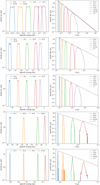 |
Fig. 4. Specific energy distributions (left) and corresponding mass return rate distributions (right) of TDEs with M = 10 M⊙, R = 5 R⊙ for β = 1–5, from top to bottom. The colours correspond to different eccentricities of the simulation as shown in the legend. Each plot corresponds to the debris after disruption at first passage and at second passage through rp. |
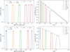 |
Fig. 5. Specific energy distributions (left) and corresponding mass return rate distributions (right) of TDEs with M = 1 M⊙, R = 1 R⊙ for β = 1 (top) and β = 2 (bottom). The colours correspond to different eccentricities of the simulation as shown in the legend. Each plot corresponds to the debris after disruption at first passage and at second passage through rp. |
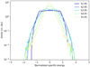 |
Fig. 6. Specific energy distribution of models S1.95, S2.95, S3.95, S4.95, and S5.95. The distributions are normalised with respect to the energy in order to compare the energy spread. The colours correspond to different β. |
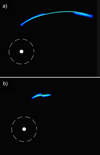 |
Fig. 7. Fallback phase of the debris after the first passage to rp from two TDEs. At low β, the typical stretching and fallback of the leading tail, which is in a deeper potential with respect to the second tail, is shown in panel a. The situation is different for higher β, where the tails both sit in deep potential and cannot stretch, resulting in a more compact clump, as shown in panel b. |
In order to see how the time evolution of the energy distribution changes with β, in Fig. 3 we compare S1.6 (top panel) to S3.8 (bottom panel). At higher β, we can observe a shift in the specific energy distribution at later times with respect to the distribution at ra and first passage to rp. However, at β = 1, all the distributions are symmetric with respect to the central value over time; as β is increased, there is a shift towards higher energies of the distributions at later times. The shift may be due to a stronger torque felt by the star with higher β.
The mass return rate distributions are shown in the right-hand panels of Figs. 4 and 5. After the star is disrupted at first passage at rp, the debris forms two tails, which stretch when falling back (Fig. 2, panels b and c). The tail that falls back first, with lower energy, translates to the rising part of the mass return rate distribution. The stretched debris that follows the leading tail translates to the t−5/3 power-law curve of the mass return rate distribution; it becomes longer as eccentricity increases with fixed β, the most noticeable examples being models with β = 1 (first rows of Figs. 4 and 5). Finally, the second debris tail at higher energy, which is the last to fall back, translates into the decrease in the fallback rate. For low eccentricity, the fallback timescales of both debris tails are similar, while for higher eccentricities the timescale for the second tail fallback is longer. We note that it is not evident how the canonical assumption that  should hold at late stages of the TDE (Lodato & Rossi 2011) when the circular disc forms due to circularisation processes.
The central peak present in the specific energy distribution in models S1.95 and S1.99 is also slightly visible in the mass return rate distribution. This is not the case for s1.95 or s1.99.
Regarding the duration of TDEs, we find that for TDEs with e = 0.99 (i.e. S1.99 and s1.99), the mass return rate distribution behaves as is expected from the parabolic one, lasting for months to years. For β = 1, at lower eccentricities (except s1.6 and s1.7), the duration is approximately a few days to a few months, but the rate is higher. If translated to a lightcurve assuming that  is valid (Lodato & Rossi 2011), these TDEs would be hard to catch observationally because they would appear as short peaks. If they were to occur in active galaxies, then they could be hidden as AGN variability, making them even more difficult to observe; however, this assertion needs considerations on the duration with respect to the variability and on the relative luminosity. The detectability situation becomes even worse for β ≥ 2, as the duration is of the order of ≲1 day.
Finally, a comparison between S-like stars and solar-like stars shows that TDEs produced by an MBH like Sgr A* are similar in duration, as can be expected since the main timescale behind a TDE depends on the mass of the MBH. We note that TDEs produced by S stars are likely to have a higher peak since more stellar mass contributes to the mass return rate.
3.2. Circularisation
There are different mechanisms that allow the debris to dissipate kinetic energy and to circularise (Evans & Kochanek 1989; Kochanek 1994). When the star is disrupted, the debris obtains a range of inclinations and their orbits will be vertically focused, intersecting close to pericentre. As a result of the strong compression at this point, a pancake shock is generated. Upon returning to pericentre, relativistic apsidal precession contributes to debris self-crossing, generating shocks due to the head of the debris colliding with its tail, which is still falling back. Another effect that occurs is shearing due to the radial focusing of the debris. Their orbits have a small range of rp and a wide range of ra, resulting in the debris going through a nozzle. In addition, the debris also has a range of apsidal angles and eccentricities, which shear the stellar material.
In general, we observe two behaviours of the circularisation of the stellar debris, depending on the initial orbital parameters e and β: (a) shocks and higher precessing angles allow the debris to form a circular disc quickly and (b) the shocks are not impactful enough to allow fast circularisation and, as a consequence, the debris follows elliptical orbits. We find that we can distinguish four different ways the debris can circularise and form a disc: type 1, the debris does not circularise efficiently and a disc is not formed or is formed after relatively long time (e.g. S1.6, Fig. 8); type 2, the debris slowly circularises and eventually forms a disc with no debris falling back (e.g. S1.8, Fig. 2); type 3, the debris circularises relatively quickly and forms a disc while there is still debris falling back (e.g. S1.95, Fig. 9); type 4, the debris quickly and efficiently circularises, mainly through self-crossings and shocks, and forms a disc with no debris falling back (e.g. S3.8, Fig. 10).
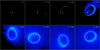 |
Fig. 8. Sequence of snapshots of model S1.6. |
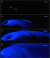 |
Fig. 9. Sequence of snapshots of model S1.95. |
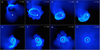 |
Fig. 10. Sequence of snapshots of model S3.8. |
For S-like stars, we observe that, for β = 1, we can identify a dividing value of the initial stellar eccentricity e = 0.8; models S1.6, S1.7, and S1.8 show a transition from type 1 to type 2, while models S1.9 and S1.95 are type 3 (we could not identify the type for S1.99 since circularisation starts at very late times and would require very long computational time). Models with β = 2 are also divided at e = 0.8 but with the difference that models S2.5, S2.6, S2.7, and S2.8 show a transition from type 1 to type 4, while models S2.9 and S2.95 are type 2. For higher β, the dividing value e = 0.8 becomes less important, as the models show a behaviour of type 4.
On the other hand, for solar-like stars we observe that the dividing value for β = 1 is e = 0.7 with models s1.6 and s1.7 being type 1, models s1.8, s1.9, and s1.95 being type 2, and model s1.99 being type 3. Lastly, for β = 2, models s2.5, s2.6, and s2.7 show transition from type 1 to type 4, while s2.8, s2.9, and s2.95 are type 4.
We analysed the identified circularisation types by using angular momentum from Eq. (3) and eccentricity, which we can calculate considering that each stellar fluid element has its own specific energy (Eq. (2)) and angular momentum after disruption:
 (11)
(11)
In Fig. 11, the debris eccentricity distributions (top row) and the angular momentum distribution (bottom row) are shown at different times for models S1.6, S1.7, and S1.8, which show a transition from type 1 to type 2. For S1.7 in particular, circularisation begins modifying the angular momentum of the debris, lowering the eccentricities (transition from type 1 to type 2), while for S1.6 little to no shock contributes and hence the debris follows the initial distribution of eccentricities (type 1). For S1.8, this effect is more evident and the shift to lower eccentricities occurs more efficiently, allowing a disc to form more easily (type 2).
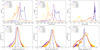 |
Fig. 11. Eccentricity distributions (top row) and angular momentum distributions (bottom row) for models S1.6, S1.7, and S1.8. For each plot the evolution of the corresponding distribution is shown for different times t (at t = 0 the star is at ra). |
We also analysed how the circularisation process changes with the orbital parameters β and e by calculating the evolution over time of the average specific energy relative to ϵcirc, later defined in Eq. (13). In the left-hand panel of Fig. 12, we plot all models with β = 3 and we observe a drop in average specific energy that becomes steeper for increasing eccentricity from e = 0.6 to 0.9 and then becomes slightly shallower for e = 0.95.
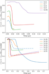 |
Fig. 12. Average specific energy relative to circularisation energy of all models with β = 3 (top) and with initial orbital eccentricity e = 0.95 (bottom). |
This behaviour is also found for β = 1, 2 for S-like stars and only for β = 1 for solar-like stars. The shallower drop observed for e = 0.95 is also observed for e = 0.99 (S1.99 and s1.99). The drop comes from the orbital energy dissipated during debris self-crossings and the generated shocks. This behaviour is consistent with results observed in previous simulations (e.g. Hayasaki et al. 2013). The increase in drop steepness with eccentricity is related to the relativistic precession acting more effectively for more eccentric orbits, thus allowing self-crossing to occur sooner after passage at rp. This means that the head will shock into the infalling tail more violently. In addition, this mechanism becomes more effective with increasing β, as shown in the right-hand panel of Fig. 12. We note that for β = 4 and 5 for S-like stars and β = 2 for solar-like stars, a shallower drop is not observed for e = 0.95. Indeed, these TDEs have been identified as having type 4 behaviour.
Once the debris goes through the circularisation mechanism as described above, it will eventually form a disc, which is generally thought to be responsible for the emission we observe. In order to analyse the disc formed by circularisation, a characteristic radius and specific energy, rcirc and ϵcirc, respectively, can be derived (Bonnerot et al. 2016) as
![Mathematical equation: $$ \begin{aligned} r_{\rm circ} = \frac{r^4_a v^2_a + \sqrt{r^4_a v^2_a[-12GM_{\rm BH}(r_a-2r_{\rm g})^2r_{\rm g} + r^4_a v^2_a]}}{2GM_{\rm BH}(r_a - 2r_{\rm g})^2} , \end{aligned} $$](/articles/aa/full_html/2020/10/aa37641-20/aa37641-20-eq15.gif) (12)
(12)
 (13)
(13)
In the literature, it is typically found that if all the fluid elements were able to circularise while conserving a common angular momentum equal to that of the star,  , then the final disc would be a ring with
  . We calculated rcirc using Eq. (12) and compared it to the tidal radius rt (see Table 1, last two columns). We find that when the disc forms, the radius is approximately equal to the estimated radius for β = 1 and eccentricity is close to parabolic (S1.95, S1.99, s1.9, s1.95, and s1.99). This estimate does not hold for lower eccentricities and β > 1. In addition, over time the disc radius in our simulations can increase (Fig. 9, panels c and d), differing from the estimated radius. More detailed simulations by Bonnerot & Lu (2020) find that the trajectories of the gas within the disc span a large range of radii because angular momentum gets efficiently redistributed amongst the debris through multiple shocks. Thus, the commonly made assumption that rcirc = 2rt is only expected if the angular momentum exchange is negligible from the stellar disruption onwards; Bonnerot & Lu (2020), for example, find that this is not the case, supporting our results.
We analysed the behaviour of the disc by studying the evolution of angular momenta of the debris before and after disc formation. In Fig. 13, we show examples with models s1.95, S1.95, and S3.8. The left-hand panel of Fig. 13 shows the angular momentum distribution of s1.95 (type 2). Here the debris is spread over a wider range of angular momenta until it all forms the disc at t ≈ 10 000 (yellow line). A different case is shown in the middle panel of Fig. 13, where we show the angular momentum distribution of S3.8 (type 4, Fig. 10). The debris undergoes strong and frequent self-crossings and shocks, and the angular momenta span over a similar range throughout the circularisation process. Finally, the angular momentum distribution of S1.95 (type 3, Fig. 9) in the right-hand panel of Fig. 13 shows that a circular disc is already formed at t = 6000 (peak centred around 0.85 l/l*) while most of the debris is still falling back, which has similar angular momenta ranging between ∼ 1.2 and 1.4 l/l*. The debris configuration at t = 8000, 12 000, and 14 000 is similar; however, the angular momentum of the disc is increasing.
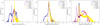 |
Fig. 13. Angular momentum distribution for models S1.95, s1.95, and S3.8. For each plot the evolution of the distribution is shown at different times t (at t = 0 the star is at the apocentre). |
In type 3 TDEs, we observe disc formation while there is still debris falling back, as also seen from the angular momentum distribution. In model S1.95, the bound debris falling back on elliptical trajectories, with ra of the order of the initial stellar orbit, has a range of angular momenta and forms an “elliptical shaped disc”, as seen in Fig. 9. In order to form this accretion flow, the bound debris needs to lose a significant amount of energy. As suggested by Piran et al. (2015), the energy thus liberated during disc formation may power the optical TDE candidates rather than the energy coming from the accretion disc itself. Furthermore, it is a common idea to consider circular accretion as an efficient radiation source to power TDEs, since it was successfully applied as the Shakura & Sunyaev (1973) model to power AGNs. However, the recent TDE observational data do not show such high energetic efficiencies, and simulations show that most of the debris stays on eccentric orbits for long times. As demonstrated by Svirski et al. (2017), high accretion flows may radiate little enough to explain the relatively small radiation fluence observed from TDE candidates. It is not clear, however, how this would affect the resulting lightcurve.
4. Conclusions
In order to fully exploit TDEs as a tool to investigate otherwise quiescent MBHs, their dynamics should be better understood. Here we study TDEs that may be produced in an environment similar to the inner parsecs of our GC. We simulated TDEs with a wide range of orbital parameters, e and β.
Our main findings are the following:
-
The dm/dϵ distributions show two features: a peak around the central value, which flattens as eccentricity decreases, and two lateral peaks called wings, related to debris tail formation.
-
The dm/dt distributions show a similar fallback timescale of the debris tails at low eccentricities, while for higher eccentricities the tail following the head has longer fallback periods. This directly affects the duration of a TDE, making those with higher eccentricities longer and more likely to be observed. Comparing TDEs produced by solar-like stars and S-like stars with the same eccentricities, we find that they have similar durations; however, S-like stars have higher dm/dt distributions than solar-like stars, as expected since their masses are larger.
-
We identify four types of circularisation evolution: the debris does not circularise efficiently and a disc is not formed or is formed after a relatively long time (type 1); the debris slowly circularises and eventually forms a disc with no debris falling back (type 2); the debris circularises relatively quickly and forms a disc while there is still debris falling back (type 3); the debris quickly and efficiently circularises, mainly through self-crossings and shocks, and forms a disc with no debris falling back (type 4).
-
In general, we find rcirc ≠ 2rt, as also shown by Bonnerot & Lu (2020). We find that the relation only holds for β = 1 and eccentricities close to parabolic.
The identification of four different types of debris evolution is dependent on the mechanisms and processes involved during circularisation. We find that for β = 1, if we increase the initial orbital eccentricity, there is a transition from a non-efficient situation (type 1), where the disc is not likely to form in a short time, to a situation where relativistic apsidal precession and debris shocks begin to play a role, leading to disc formation (types 2 and 3). On the other hand, an increase in the penetration factor leads to more impactful self-crossings and shocks, which allow a quick and efficient circularisation of the debris (type 4). The behaviour of S stars and solar-like stars is almost similar for β = 1, while for β = 2 TDEs of solar-like stars evolve as type 4 instead of type 2, meaning that for these stars the debris is all circularised when the disc is formed. In type 4 TDEs, stellar debris is accreted quickly into the MBH, mostly during the self-crossing and shock processes, whereas for type 3 the accretion is more moderate. In these respects, less debris is available for the disc in type 4 than in type 3.
We find the difference between TDEs of S-like stars and solar-like stars during observations in their fallback mass rate and peak luminosities. Our models assume stars with a polytropic index γ = 5/3; while polytropes might be a good first order approximation, they do not describe the detailed structure of density profiles of different stellar types well. A more detailed analysis would require more realistic stellar models. Indeed, Golightly et al. (2019b), who ran simulations of stars on parabolic orbits and β = 3 using more realistic stellar models from MESA code Paxton et al. (2011), find that there are significant differences in fallback rates when using stars with different masses and ages, leading to deviations from predictions based on simple polytropic models.
Due to computational costs, we chose to model a non-spinning MBH. However, there is observational evidence that in many cases MBHs are spinning. The presence of a Kerr MBH introduces the Lense-Thirring effect and nodal precession, in addition to relativistic apsidal precession. While the latter induces debris stream self-crossings and rapid circularisation, nodal precession may hinder them by putting debris streams on different orbital planes. Dai et al. (2013), Hayasaki et al. (2016), and Liptai et al. (2019) have investigated the effects of a Kerr MBH on a TDE. In general, the effect of nodal precession is to delay circularisation and disc formation, but it does not prevent it. In particular, Hayasaki et al. (2016) and Liptai et al. (2019) investigated the effects of the MBH spin on the formation of a thick disc and a thin ring. Spin dependence is mostly absent in the case of a thick disc, while it is important for the circularisation of thin debris streams where retrograde or aligned spin can aid the process. On the other hand, the process is hindered by prograde or misaligned spin (Hayasaki et al. 2016). Liptai et al. (2019) find that disc formation is robust with respect to initial stellar orbit inclination and MBH spin. They also find that self-crossings are inhibited only during the first orbit, thus only introducing a short delay in the case of orbit prograde with respect to the MBH spin. In addition, depending on the inclination, Liptai et al. (2019) find that simulations are brighter by ∼1 order of magnitude in early stages, and discs are formed ∼1 orbital period earlier. It should be noted that while Hayasaki et al. (2016) performed simulations with β = 1 and 2, all but one of the Liptai et al. (2019) simulations have β = 5. Thus, a relatively short delay in circularisation may be introduced in our study case, depending on whether the stellar orbit is prograde or retrograde (also considering that a fraction of young stars found in the GC are orbiting clockwise and others anti-clockwise, and that there is a warped disc).
Thus, the next step in characterising TDEs that could occur in similar galactic environments as our GC is to study TDEs with different orbital parameters β and e (as found in the GC), also taking into account the MBH spin, and to use realistic stellar models of different types of stars found in such environments. Such a study could provide better insight not only into the MBH responsible for the disruption, but also into the type of disrupted star, thus allowing us to learn more about the innermost stellar populations of far galaxies, otherwise difficult to observe directly.
The code is publicly available at https://phantomsph.bitbucket.io/
Acknowledgments
A. C. and A. G. acknowledge the financial support from the Slovenian Research Agency (Grants P1-0031, I0-0033, and J1-8136) and networking support by COST Actions CA16104 GWverse and CA16214 PHAROS. A. C. also acknowledges Arctur d.o.o. for providing their computational resources.
References
- Alexander, T. 2005, Phys. Rep., 419, 65 [NASA ADS] [CrossRef] [Google Scholar]
- Antonini, F., Lombardi, J. C. Jr., & Merritt, D. 2011, ApJ, 731, 128 [CrossRef] [Google Scholar]
- Arcavi, I., Gal-Yam, A., Sullivan, M., et al. 2014, ApJ, 793, 38 [NASA ADS] [CrossRef] [Google Scholar]
- Ayal, S., Livio, M., & Piran, T. 2000, ApJ, 545, 772 [NASA ADS] [CrossRef] [Google Scholar]
- Bade, N., Komossa, S., & Dahlem, M. 1996, A&A, 309, L35 [NASA ADS] [Google Scholar]
- Blagorodnova, N., Cenko, S. B., Kulkarni, S. R., et al. 2019, ApJ, 873, 92 [CrossRef] [Google Scholar]
- Bloom, J. S., Giannios, D., Metzger, B. D., et al. 2011, Science, 333, 203 [CrossRef] [PubMed] [Google Scholar]
- Bogdanović, T., Cheng, R. M., & Amaro-Seoane, P. 2014, ApJ, 788, 99 [CrossRef] [Google Scholar]
- Bonnerot, C., & Lu, W. 2020, MNRAS, 495, 1374 [CrossRef] [Google Scholar]
- Bonnerot, C., Rossi, E. M., Lodato, G., & Price, D. J. 2016, MNRAS, 455, 2253 [NASA ADS] [CrossRef] [Google Scholar]
- Brown, W. R. 2015, ARA&A, 53, 15 [Google Scholar]
- Brown, G. C., Levan, A. J., Stanway, E. R., et al. 2015, MNRAS, 452, 4297 [NASA ADS] [CrossRef] [Google Scholar]
- Cannizzo, J. K., Lee, H. M., & Goodman, J. 1990, ApJ, 351, 38 [NASA ADS] [CrossRef] [Google Scholar]
- Carter, B., & Luminet, J. P. 1983, A&A, 121, 97 [Google Scholar]
- Cenko, S. B., Krimm, H. A., Horesh, A., et al. 2012, ApJ, 753, 77 [NASA ADS] [CrossRef] [Google Scholar]
- Chornock, R., Berger, E., Gezari, S., et al. 2014, ApJ, 780, 44 [NASA ADS] [CrossRef] [Google Scholar]
- Coughlin, E. R., & Nixon, C. 2015, ApJ, 808, L11 [NASA ADS] [CrossRef] [Google Scholar]
- Coughlin, E. R., Nixon, C., Begelman, M. C., & Armitage, P. J. 2016a, MNRAS, 459, 3089 [CrossRef] [Google Scholar]
- Coughlin, E. R., Nixon, C., Begelman, M. C., Armitage, P. J., & Price, D. J. 2016b, MNRAS, 455, 3612 [NASA ADS] [CrossRef] [Google Scholar]
- Dai, L., Escala, A., & Coppi, P. 2013, ApJ, 775, L9 [CrossRef] [Google Scholar]
- Donley, J. L., Brandt, W. N., Eracleous, M., & Boller, T. 2002, AJ, 124, 1308 [NASA ADS] [CrossRef] [Google Scholar]
- Englmaier, P., & Shlosman, I. 2004, ApJ, 617, L115 [NASA ADS] [CrossRef] [Google Scholar]
- Eisenhauer, F., Genzel, R., Alexander, T., et al. 2005, ApJ, 628, 246 [NASA ADS] [CrossRef] [Google Scholar]
- Evans, C. R., & Kochanek, C. S. 1989, ApJ, 346, L13 [NASA ADS] [CrossRef] [Google Scholar]
- Gezari, S., Martin, D. C., Milliard, B., et al. 2006, ApJ, 653, L25 [NASA ADS] [CrossRef] [Google Scholar]
- Gezari, S., Basa, S., Martin, D. C., et al. 2008, ApJ, 676, 944 [NASA ADS] [CrossRef] [Google Scholar]
- Gezari, S., Chornock, R., Rest, A., et al. 2012, Nature, 485, 217 [NASA ADS] [CrossRef] [PubMed] [Google Scholar]
- Ghez, A. M., Duchêne, G., Matthews, K., et al. 2003, ApJ, 586, L127 [NASA ADS] [CrossRef] [Google Scholar]
- Gillessen, S., Eisenhauer, F., Trippe, S., et al. 2009, ApJ, 692, 1075 [NASA ADS] [CrossRef] [Google Scholar]
- Gingold, R. A., & Monaghan, J. J. 1977, MNRAS, 181, 375 [Google Scholar]
- Golightly, E. C. A., Coughlin, E. R., & Nixon, C. J. 2019a, ApJ, 872, 163 [CrossRef] [Google Scholar]
- Golightly, E. C. A., Nixon, C. J., & Coughlin, E. R. 2019b, ApJ, 882, L26 [CrossRef] [Google Scholar]
- Gomboc, A., & Čadež, A. 2005, ApJ, 625, 278 [NASA ADS] [CrossRef] [Google Scholar]
- Guillochon, J., & Ramirez-Ruiz, E. 2013, ApJ, 767, 25 [NASA ADS] [CrossRef] [Google Scholar]
- Guillochon, J., Ramirez-Ruiz, E., Rosswog, S., & Kasen, D. 2009, ApJ, 705, 844 [NASA ADS] [CrossRef] [Google Scholar]
- Habibi, M., Gillessen, S., Martins, F., et al. 2017, ApJ, 847, 120 [NASA ADS] [CrossRef] [Google Scholar]
- Halpern, J. P., Gezari, S., & Komossa, S. 2004, ApJ, 604, 572 [NASA ADS] [CrossRef] [Google Scholar]
- Hamers, A. S., & Perets, H. B. 2017, ApJ, 846, 123 [CrossRef] [Google Scholar]
- Hayasaki, K., Stone, N., & Loeb, A. 2013, MNRAS, 434, 909 [NASA ADS] [CrossRef] [Google Scholar]
- Hayasaki, K., Stone, N., & Loeb, A. 2016, MNRAS, 461, 3760 [NASA ADS] [CrossRef] [Google Scholar]
- Hills, J. G. 1988, Nature, 331, 687 [Google Scholar]
- Holoien, T. W. S., Prieto, J. L., Bersier, D., et al. 2014, MNRAS, 445, 3263 [NASA ADS] [CrossRef] [Google Scholar]
- Holoien, T. W. S., Kochanek, C. S., Prieto, J. L., et al. 2016, MNRAS, 455, 2918 [NASA ADS] [CrossRef] [Google Scholar]
- Holoien, T. W. S., Huber, M. E., Shappee, B. J., et al. 2019, ApJ, 880, 120 [CrossRef] [Google Scholar]
- Ivanov, P. B., & Novikov, I. D. 2001, ApJ, 549, 467 [NASA ADS] [CrossRef] [Google Scholar]
- Karas, V., & Šubr, L. 2007, A&A, 470, 11 [NASA ADS] [CrossRef] [EDP Sciences] [Google Scholar]
- Kesden, M. 2012, Phys. Rev. D, 86, 064026 [CrossRef] [Google Scholar]
- Khabibullin, I., & Sazonov, S. 2014, MNRAS, 444, 1041 [NASA ADS] [CrossRef] [Google Scholar]
- Kobayashi, S., Laguna, P., Phinney, E. S., & Mészáros, P. 2004, ApJ, 615, 855 [NASA ADS] [CrossRef] [Google Scholar]
- Kochanek, C. S. 1994, ApJ, 422, 508 [NASA ADS] [CrossRef] [Google Scholar]
- Komossa, S. 2015, J. High Energy Astrophys., 7, 148 [Google Scholar]
- Komossa, S., & Bade, N. 1999, in The Giant X-ray Outburst in NGC 5905 - a Tidal Disruption Event?, eds. J. Poutanen, & R. Svensson, ASP Conf. Ser., 161, 234 [Google Scholar]
- Komossa, S., & Greiner, J. 1999, A&A, 349, L45 [NASA ADS] [Google Scholar]
- Kosovichev, A. G., & Novikov, I. D. 1992, MNRAS, 258, 715 [NASA ADS] [CrossRef] [Google Scholar]
- Lacy, J. H., Townes, C. H., & Hollenbach, D. J. 1982, ApJ, 262, 120 [NASA ADS] [CrossRef] [Google Scholar]
- Laguna, P., Miller, W. A., Zurek, W. H., & Davies, M. B. 1993, ApJ, 410, L83 [NASA ADS] [CrossRef] [Google Scholar]
- Liptai, D., Price, D. J., Mandel, I., & Lodato, G. 2019, MNRAS, submitted [arXiv:1910.10154] [Google Scholar]
- Lodato, G., & Rossi, E. M. 2011, MNRAS, 410, 359 [NASA ADS] [CrossRef] [Google Scholar]
- Lodato, G., King, A. R., & Pringle, J. E. 2009, MNRAS, 392, 332 [NASA ADS] [CrossRef] [Google Scholar]
- Loeb, A., & Ulmer, A. 1997, ApJ, 489, 573 [NASA ADS] [CrossRef] [Google Scholar]
- Lucy, L. B. 1977, AJ, 82, 1013 [NASA ADS] [CrossRef] [Google Scholar]
- Luminet, J. P., & Marck, J. A. 1985, MNRAS, 212, 57 [CrossRef] [MathSciNet] [Google Scholar]
- Magorrian, J., & Tremaine, S. 1999, MNRAS, 309, 447 [NASA ADS] [CrossRef] [Google Scholar]
- Merritt, D., & Poon, M. Y. 2004, ApJ, 606, 788 [NASA ADS] [CrossRef] [Google Scholar]
- Monaghan, J. J. 1992, ARA&A, 30, 543 [NASA ADS] [CrossRef] [Google Scholar]
- Nolthenius, R. A., & Katz, J. I. 1982, ApJ, 263, 377 [NASA ADS] [CrossRef] [Google Scholar]
- Parsa, M., Eckart, A., Shahzamanian, B., et al. 2017, ApJ, 845, 22 [NASA ADS] [CrossRef] [Google Scholar]
- Paxton, B., Bildsten, L., Dotter, A., et al. 2011, ApJS, 192, 3 [Google Scholar]
- Perets, H. B., Hopman, C., & Alexander, T. 2007, ApJ, 656, 709 [NASA ADS] [CrossRef] [Google Scholar]
- Phinney, E. S. 1989, in The Center of the Galaxy, ed. M. Morris, IAU Symp., 136, 543 [NASA ADS] [CrossRef] [Google Scholar]
- Piran, T., Svirski, G., Krolik, J., Cheng, R. M., & Shiokawa, H. 2015, ApJ, 806, 164 [NASA ADS] [CrossRef] [Google Scholar]
- Price, D. J. 2007, PASA, 24, 159 [Google Scholar]
- Price, D. J., Wurster, J., Tricco, T. S., et al. 2018, PASA, 35, e031 [Google Scholar]
- Rees, M. J. 1988, Nature, 333, 523 [NASA ADS] [CrossRef] [Google Scholar]
- Rosswog, S., Ramirez-Ruiz, E., & Hix, W. R. 2009, ApJ, 695, 404 [NASA ADS] [CrossRef] [Google Scholar]
- Shakura, N. I., & Sunyaev, R. A. 1973, A&A, 500, 33 [NASA ADS] [Google Scholar]
- Shen, R.-F., & Matzner, C. D. 2014, ApJ, 784, 87 [CrossRef] [Google Scholar]
- Shiokawa, H., Krolik, J. H., Cheng, R. M., Piran, T., & Noble, S. C. 2015, ApJ, 804, 85 [NASA ADS] [CrossRef] [Google Scholar]
- Shlosman, I., Frank, J., & Begelman, M. C. 1989, Nature, 338, 45 [NASA ADS] [CrossRef] [Google Scholar]
- Stone, N., & Loeb, A. 2011, in American Astronomical Society Meeting Abstracts #218, Am. Astron. Soc. Meeting Abstr., 218, 235.04 [Google Scholar]
- Stone, N. C., & Metzger, B. D. 2016, MNRAS, 455, 859 [NASA ADS] [CrossRef] [Google Scholar]
- Stone, N. C., & van Velzen, S. 2016, ApJ, 825, L14 [NASA ADS] [CrossRef] [Google Scholar]
- Stone, N., Sari, R., & Loeb, A. 2013, MNRAS, 435, 1809 [NASA ADS] [CrossRef] [Google Scholar]
- Strubbe, L. E., & Quataert, E. 2009, MNRAS, 400, 2070 [NASA ADS] [CrossRef] [Google Scholar]
- Svirski, G., Piran, T., & Krolik, J. 2017, MNRAS, 467, 1426 [Google Scholar]
- Tejeda, E., & Rosswog, S. 2013, MNRAS, 433, 1930 [CrossRef] [Google Scholar]
- Wang, J., & Merritt, D. 2004, ApJ, 600, 149 [NASA ADS] [CrossRef] [Google Scholar]
- Yusef-Zadeh, F., & Wardle, M. 2012, J. Phys. Conf. Ser., 372, 012024 [CrossRef] [Google Scholar]
- Yusef-Zadeh, F., Melia, F., & Wardle, M. 2000, Science, 287, 85 [NASA ADS] [CrossRef] [Google Scholar]
All Tables
All Figures
|
Fig. 1. Orbits with eccentricities ranging from e = 0.6 to 0.95 with fixed β = 1 (a), and orbits with penetration ranging from β = 1 to 5 with fixed e = 0.8 (b). Each orbit is the trajectory of the centre of mass of a star in the generalised Newtonian potential (Eq. (1)) in one period. The filled circle represents the rISCO, while the dashed circle represents the rt. |
| In the text | |
|
Fig. 2. Sequence of snapshots of model S1.8. The MBH is represented by the full white circle, which has a radius equal to rISCO, while the dashed white line represents the tidal radius rt. In panel a, the star is in its initial position ra and orbits the MBH on an anti-clockwise trajectory. In panel b, the star has been disrupted and the debris formed two tails, which will stretch and fall back (panel c). In panels d–g, the debris is going through circularisation processes, which result in the formation of a disc (panel h). |
| In the text | |
|
Fig. 3. Specific energy distribution (left) and corresponding fallback mass rates (right) of models S1.6 (top) and S3.8 (bottom). The colours correspond to different times of the simulation: blue is at the star’s initial position at ra, orange is at the first passage to rp, green is during the formation of the two debris tails, red is during the stretching and falling back of the most bound debris tail, and purple is at the second passage to rp. |
| In the text | |
|
Fig. 4. Specific energy distributions (left) and corresponding mass return rate distributions (right) of TDEs with M = 10 M⊙, R = 5 R⊙ for β = 1–5, from top to bottom. The colours correspond to different eccentricities of the simulation as shown in the legend. Each plot corresponds to the debris after disruption at first passage and at second passage through rp. |
| In the text | |
|
Fig. 5. Specific energy distributions (left) and corresponding mass return rate distributions (right) of TDEs with M = 1 M⊙, R = 1 R⊙ for β = 1 (top) and β = 2 (bottom). The colours correspond to different eccentricities of the simulation as shown in the legend. Each plot corresponds to the debris after disruption at first passage and at second passage through rp. |
| In the text | |
|
Fig. 6. Specific energy distribution of models S1.95, S2.95, S3.95, S4.95, and S5.95. The distributions are normalised with respect to the energy in order to compare the energy spread. The colours correspond to different β. |
| In the text | |
|
Fig. 7. Fallback phase of the debris after the first passage to rp from two TDEs. At low β, the typical stretching and fallback of the leading tail, which is in a deeper potential with respect to the second tail, is shown in panel a. The situation is different for higher β, where the tails both sit in deep potential and cannot stretch, resulting in a more compact clump, as shown in panel b. |
| In the text | |
|
Fig. 8. Sequence of snapshots of model S1.6. |
| In the text | |
|
Fig. 9. Sequence of snapshots of model S1.95. |
| In the text | |
|
Fig. 10. Sequence of snapshots of model S3.8. |
| In the text | |
|
Fig. 11. Eccentricity distributions (top row) and angular momentum distributions (bottom row) for models S1.6, S1.7, and S1.8. For each plot the evolution of the corresponding distribution is shown for different times t (at t = 0 the star is at ra). |
| In the text | |
|
Fig. 12. Average specific energy relative to circularisation energy of all models with β = 3 (top) and with initial orbital eccentricity e = 0.95 (bottom). |
| In the text | |
|
Fig. 13. Angular momentum distribution for models S1.95, s1.95, and S3.8. For each plot the evolution of the distribution is shown at different times t (at t = 0 the star is at the apocentre). |
| In the text | |
Current usage metrics show cumulative count of Article Views (full-text article views including HTML views, PDF and ePub downloads, according to the available data) and Abstracts Views on Vision4Press platform.
Data correspond to usage on the plateform after 2015. The current usage metrics is available 48-96 hours after online publication and is updated daily on week days.
Initial download of the metrics may take a while.