| Issue |
A&A
Volume 640, August 2020
|
|
|---|---|---|
| Article Number | A24 | |
| Number of page(s) | 7 | |
| Section | Astrophysical processes | |
| DOI | https://doi.org/10.1051/0004-6361/202037471 | |
| Published online | 04 August 2020 | |
Accurate analytic formula for light bending in Schwarzschild metric
1
Department of Physics and Astronomy, University of Turku, 20014 Turku, Finland
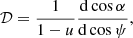
e-mail: This email address is being protected from spambots. You need JavaScript enabled to view it.
2
Space Research Institute of the Russian Academy of Sciences, Profsoyuznaya Str. 84/32, 117997 Moscow, Russia
3
Nordita, KTH Royal Institute of Technology and Stockholm University, Roslagstullsbacken 23, 10691 Stockholm, Sweden
Received:
9
January
2020
Accepted:
24
June
2020
Abstract
We propose new analytic formulae describing light bending in the Schwarzschild metric. For an emission radii above the photon orbit at the 1.5 Schwarzschild radius, the formulae have an accuracy of better than 0.2% for the bending angle and 3% for the lensing factor for any trajectories that turn around a compact object by less than about 160°. In principle, they can be applied to any emission point above the horizon of the black hole. The proposed approximation can be useful for problems involving emission from neutron stars and accretion discs around compact objects when fast accurate calculations of light bending are required. It can also be used to test the codes that compute light bending using exact expressions via elliptical integrals.
Key words: accretion, accretion disks / black hole physics / methods: numerical / X-rays: binaries / stars: black holes / stars: neutron
© ESO 2020
1. Introduction
Understanding the physical processes in the vicinity of black holes (BHs) and neutron stars (NSs) requires a detailed treatment of light propagation from a compact source to the distant observer. In a general case of a rotating compact object, this is a complex, numerically extensive problem (e.g. Dexter 2016; Nättilä & Pihajoki 2018). For a slowly rotating object, the Schwarzschild metric can be used; however, even in this case, numerical, time-consuming evaluations of elliptical integrals that can be used to describe light bending are needed. The situation becomes acute when one needs to fit the data with a model varying many parameters, which may require thousands, if not millions, of iterations. Such a problem exists, for example, when trying to determine NS parameters from the pulse form observed from millisecond pulsars which have an oblate shape (Miller & Lamb 2015; Watts et al. 2016; Bogdanov et al. 2019; Riley et al. 2019; Miller et al. 2019).
In many applications, the position of the emission point is defined, for example, by the radius-vector R and by the azimuthal angle ψ vector R makes with the direction to the observer (see Fig. 1). We then need to compute the emission angle α that the photon trajectory makes with R. In order to do so, we would have to tabulate ψ(α) at a grid of radii R, then reverse the dependence to α(ψ), and finally interpolate in the resulting tables to find α for given R and ψ. An analytical formula for α(R, ψ) would simplify and speed up calculations. It can also be used to test other, more accurate routines for light bending.
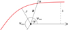 |
Fig. 1. Geometry of light bending in the Schwarzschild metric. The observer is situated on the right at ψ = 0. |
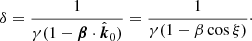
A powerful approximation to the bending integral in the Schwarzschild metric of the required form α(R, ψ) was discovered by Beloborodov (2002). He showed that there is a nearly linear relation between cos α and cos ψ:
 (1)
(1)
where u = RS/R is the compactness and RS = 2GM/c2 is the Schwarzschild radius of the central object of mass M. This approximation has a high accuracy for direct trajectories (those that do not pass through the turning point, i.e. periastron) and for compact stars of a radius exceeding 2 RS. A useful property of this approximation is that it is linear in three parameters: cos α, cos ψ, and u. Thus, for any known two parameters, the third can be found easily. For example, if we are interested in the total bending angle corresponding to a given compactness, we would fix cos α = 0, find ψmax from a simple relation cos ψmax = −u/(1 − u), and the total bending angle as 2ψmax − π. This approximation can also be used to obtain an approximate form of the photon trajectory for the given impact parameter, which depends on α and u (see Eq. (4) below), as given by Eq. (3) in Beloborodov (2002). Using a similar approach, other approximate forms for the photon trajectory and the total bending angle are suggested by Semerák (2015).
In this paper, however, we are only interested in a simple approximation for α(R, ψ). We propose the following approximation:
![Mathematical equation: $$ \begin{aligned} x = (1-u) \,y \left\{ 1 + \frac{u^2y^2}{112}- \frac{e}{100} u y \left[\ln \left(1-\frac{y}{2}\right) +\frac{y}{2}\right] \right\} , \end{aligned} $$](/articles/aa/full_html/2020/08/aa37471-20/aa37471-20-eq2.gif) (2)
(2)
where e is the base of the natural logarithm. It works for trajectories that make less than half of a full turn around a central object and for the radii all the way to the horizon. We then compare our new approximation to other approximations proposed in the literature and test it on the following two well-known problems: the light curve from two antipodal hotspots at the NS surface and the line emission from the accretion disc around a Schwarzschild BH.
2. Light bending in the Schwarzschild metric
2.1. Bending angle
Here, we consider a photon passing near a gravitating centre (BH or NS) and escaping to infinity (see Fig. 1). In the Schwarzschild metric, the shape of the photon’s trajectory is described by the following equation (Misner et al. 1973, p. 673):
 (3)
(3)
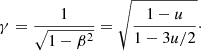
where R is the circumferential radius, ψ is the azimuthal angle, and b is the impact parameter. The impact parameter and the angle, α, between the radial direction and the photon trajectory are related by (e.g. Beloborodov 2002)
 (4)
(4)
In a BH case, a photon with an impact parameter of  (Misner et al. 1973, p. 675) may be captured by the central object. The critical impact parameter bcr corresponds to the critical emission angle
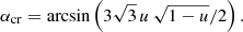 (5)
(5)
If the emission radius is small, R ≤ 1.5 RS (i.e. u ≥ 2/3), only photons with α ≤ αcr can escape to infinity. For a larger emission radius of R > 1.5 RS, all photons with α ≤ π/2 escape. In these cases, the observer angle ψ(R, α), that is, the angle between the radius vector of the emission point and the photon momentum at infinity, is given by the integral (e.g. Pechenick et al. 1983; Beloborodov 2002)
![Mathematical equation: $$ \begin{aligned} \psi (R,\alpha )=\int _R^{\infty } \frac{{\mathrm{d} r}}{r^2} \left[ \frac{1}{b^2} - \frac{1}{r^2}\left( 1- \frac{{R_{\rm S}}}{r}\right)\right]^{-1/2}, \end{aligned} $$](/articles/aa/full_html/2020/08/aa37471-20/aa37471-20-eq7.gif) (6)
(6)
where b is given by Eq. (4).
If R > 1.5 RS, the critical emission angle is instead π − αcr, and the condition for photon capture can be written as
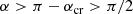 (7)
(7)
or
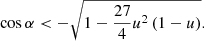 (8)
(8)
Thus, photons emitted at an angle of π/2 < α ≤ π − αcr escape, but they first pass though the turning point (see Fig. 1) at an azimuthal angle of
 (9)
(9)
The periastron, p, can be found by setting dR/dψ = 0 in Eq. (3) and solving the resulting cubic equation p3 = b2(p − RS) to get
![Mathematical equation: $$ \begin{aligned} p=-\frac{2}{\sqrt{3}}\,b \cos \left\{ [\arccos (b_{\rm cr}/b)+2\pi ]/3\right\} . \end{aligned} $$](/articles/aa/full_html/2020/08/aa37471-20/aa37471-20-eq11.gif) (10)
(10)
The observer angle is then given by
 (11)
(11)
A numerical method to accurately compute bending integrals is described, for example, by Salmi et al. (2018). The resulting relation between ψ and cos α for different radii is shown in Fig. 2. We see that ψ diverges when cos α approaches critical values. This corresponds to many rotations of a photon around the BH and may result in multiple images.
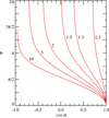 |
Fig. 2. Light bending relation between the cosine of the emission angle α and the angle ψ between the line of sight and the radius-vector of the emission point computed using exact relations (6)–(11) for the Schwarzschild metric for six different emission radii R/RS = 1.1, 1.3, 1.5, 2, 3, and 10, which are marked next to the corresponding curves. |
For the majority of realistic astrophysical situations, we can limit ourselves only to the primary image with ψ < π, because other images may be blocked by the accretion disc and the flux decreases rapidly with the number of turns (Luminet 1979). In the NS case, the trajectories that pass through the stellar surface are truncated. For a spherical star, this means that we are only interested in trajectories with cos α > 0. Rapidly rotating NSs are not spherical anymore and, in principle, some trajectories with cos α < 0 may also become possible. For the primary image, the dependence cos α(cos ψ) would be sufficient and we plotted it in Fig. 3.
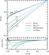 |
Fig. 3. Upper panel: light bending relation between the cosine of the emission angle α and the cosine of the angle ψ between the line of sight and the radius-vector of the emission point in the Schwarzschild metric. The red curves give the exact relation. Our new approximate relation (2) is shown with the black curves. The blue straight lines are for the Beloborodov (2002) approximation (1), while the green curves represent the approximation (16) by La Placa et al. (2019). The red, green, and black curves practically coincide. The solid, dotted, dashed, and dot-dashed curves correspond to radii R/RS = 1.5, 2, 2.5, and 3, respectively. Bottom panel: relative error of the emission angle δα/α for three approximations as compared to the exact result. Same notations as in the upper panel. |
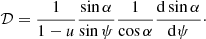
2.2. Lensing factor
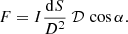
Now we turn to a problem of evaluating flux from a surface element of the area dS. Without losing a generality, we can assume that the normal to the surface is along the radial direction R. The flux observed from this element is proportional to the product of the radiation intensity I and the solid angle occupied by the element on the observer’s sky dΩ. The solid angle can be represented via the impact parameter as
 (12)
(12)
with D being the distance to the source and ϕ is the azimuthal angle in the spherical coordinate system with the z-axis directed along the line of sight. Expressing the element area as dS = R2d cos ψ dϕ and using Eq. (4), we get (Beloborodov 2002)
 (13)
(13)
We see that the solid angle has two terms: The first is just the solid angle that the element observed at inclination α would occupy in flat space dS cos α/D2, while the second factor corrects for light bending. Thus in calculations of the observed flux, it is not only important to get an accurate estimate of the emission angle α for a given ψ, but also to evaluate the lensing factor accurately
 (14)
(14)
which is shown in Fig. 4.
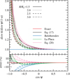 |
Fig. 4. Same as Fig. 3, but for the lensing factor 𝒟. The approximation (20) is shown by the pink curves. |
3. Approximate light bending formulae
We need to design approximations of the form α(u, ψ) and 𝒟(u, ψ). A simple approximate relation (1) discovered by Beloborodov (2002) is not very accurate for large emission angles α and large compactness u ≳ 1/2. This is demonstrated in Fig. 3, where Beloborodov (2002) approximation (blue lines) is compared with the exact relation (red curves). We see that the error of the emission angle δα/α grows systematically with decreasing cos ψ (that is increasing ψ, which corresponds to the emission points further from our line of sight). For small compactness, u ≲ 1/3 (i.e. R ≳ 3RS), and the NS case, this is not a problem because we are mostly interested in trajectories with cos α > 0, where the error does not exceed 0.7%. The error grows, however, with compactness and for u = 1/2, it is already 10%.
The situation is even worse for the lensing factor (14). Equation (1) implies 𝒟 = 1, while the exact value grows rapidly at negative cos ψ (see Fig. 4), for example at cos ψ = −0.7 (i.e. ψ = 134°), deviation from unity exceeds 10% for u = 1/3 and 15% for u = 1/2. It is thus clear that the approximation may introduce a significant error in the flux observed, for example, from a spot at the NS far side or from the accretion disc viewed at a large inclination. The realisation of this problem motivates us to look for a different, more accurate approximation.
Approximation (1) was derived by Beloborodov (2002) from the exact expression of the bending angle (6) by expanding the integral in the Taylor series over the small parameter x and obtaining a new Taylor series for y(x). Poutanen & Beloborodov (2006) got an expression for the reverse relation:
 (15)
(15)
which, however, still has the same problems as the original approximation (1) because deviations appear at large values of the argument y.
Recently, a purely phenomenological formula was proposed by La Placa et al. (2019):
![Mathematical equation: $$ \begin{aligned} x = (1-u) y \left\{ 1 + k_1 u [ 1-\cos (\psi -k_2)]^{k_3} \right\} , \end{aligned} $$](/articles/aa/full_html/2020/08/aa37471-20/aa37471-20-eq17.gif) (16)
(16)
where k1 = 0.1416, k2 = 1.196 and k3 = 2.726. This approximation is shown in Fig. 3 by the green curves. We see that it is better than 1% accurate for most of the angles of interest. However, it does not reproduce the exact behaviour well at small angles 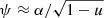 experiencing unphysical jumps, which are also reflected in the jumps in the derivative (lensing factor) at small ψ (see green curves in Fig. 4). The lensing factor has a typical accuracy of 3−5% and deviates by more than 5% from the exact values at cos ψ ≲ −0.8.
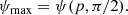
We instead suggest designing a fitting formula that keeps the correct asymptotic behaviour at ψ → 0, as given by Eq. (15), but at the same time provides a sufficient curvature when cos ψ is close to −1 (i.e. y = 2). For that, we added a logarithmic term of the type ∝ln(1 − y/2) that satisfies the second condition, but subtracted the terms of the corresponding Taylor expansion around y = 0 in order to satisfy the first condition. We found that a good fit to the exact bending relation is provided by Eq. (2). It gives an error below 0.06% for cos ψ > −0.5 (i.e. for the angle ψ < 120° from the radial direction) and any radius exceeding 1.5 RS. At these radii, the error exceeds 0.2% for cos ψ < −0.95, that is ψ > 162° (see black curves in Fig. 3), which corresponds to the emission points behind the compact object. The contours of constant errors on the plane (u, cos ψ) are shown in Fig. 5a. We see that approximation works rather well, even for radii between the event horizon and the photon orbit, RS < R < 1.5 RS (i.e. 2/3 < u < 1); of course, this is only the case for emission angles that are very close to the radial direction, so that the photon trajectory makes less than half of a full turn around a compact object.
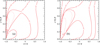 |
Fig. 5. Contours of the constant relative error on (a) the bending angle δα/α and (b) the lensing factor for our approximations given by Eqs. (2) and (17). Neighbouring contours differ by a factor of 10 in the value of the error. Solid and dotted curves represent positive and negative deviations, respectively. |
The lensing factor implied by Eq. (2),
![Mathematical equation: $$ \begin{aligned} \mathcal{D} = 1 + \frac{3u^2y^2}{112} - \frac{e}{100} u y \left[ 2\,\ln \left(1-\frac{y}{2}\right) + y\frac{1-3y/4}{1-y/2}\right], \end{aligned} $$](/articles/aa/full_html/2020/08/aa37471-20/aa37471-20-eq19.gif) (17)
(17)
also has a high accuracy. Figure 5b shows the contours of the constant error on the plane (u, cos ψ). We see that the error only exceeds 10% for cos ψ < −0.9 and u > 0.8. For an object with a radius exceeding the photon orbit (i.e. u < 2/3), the error is below 0.3% for cos ψ > −0.5 (see also the black curves in Fig. 4).
Another way to approximate the lensing factor (14) is to start from its following form
 (18)
(18)
The derivative dψ/d sin α can be written in an explicit form that follows from Eq. (6) as
![Mathematical equation: $$ \begin{aligned} \frac{\mathrm{d}\psi }{\mathrm{d}\sin \alpha } = \frac{R}{\sqrt{1-u}} \int _R^{\infty } \frac{{\mathrm{d} r}}{r^2} \left[ 1 - \frac{b^2}{r^2}\left(1- \frac{{R_{\rm S}}}{r}\right)\right]^{-3/2}. \end{aligned} $$](/articles/aa/full_html/2020/08/aa37471-20/aa37471-20-eq21.gif) (19)
(19)
By expanding it as well as sin α and cos α in Eq. (18) in a small parameter x = 1 − cosα up to x2, but keeping the factor sin ψ in the denominator, we get1
![Mathematical equation: $$ \begin{aligned} \mathcal{D} \approx \frac{\sqrt{2y}}{\sin \psi } \left[ 1- \frac{y}{4} + y^2 \left( -\frac{1}{32} + \frac{5}{224} u^2 \right)\right]\cdot \end{aligned} $$](/articles/aa/full_html/2020/08/aa37471-20/aa37471-20-eq22.gif) (20)
(20)
Here in the final expression, we used Eq. (1) and substituted x = y(1 − u) to get 𝒟 as a function of ψ, not α. The factor sin ψ in the denominator gives rise to a diverging behaviour at ψ → π (see Fig. 4), which allows us to describe the actual dependence of the lensing factor slightly better than just a constant 𝒟 = 1 from Belobodorov’s approximation, but worse than the other approximations considered above.
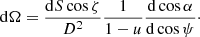
4. Applications
4.1. Hotspots at a neutron star surface
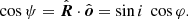
We now consider a test case which demonstrates the power of approximate formulae for light bending. We consider two antipodal spots of the area dS at a slowly rotating spherical NS of radius R and mass M where the observer unit vector is  and the co-latitude of the primary spot is θ. The unit-vector corresponding to the radius vector of the primary hotspot varies with the rotational phase φ as
  . This gives us the following expression for the angle between
  and
and  :
:
 (21)
(21)
For the secondary spot, we substituted φ → φ + π and θ → π − θ. The observed bolometric flux is F = I dΩ, where the solid angle is given by Eq. (13). Thus the flux is (Beloborodov 2002)
 (22)
(22)
If the intensity at the NS surface is angle-independent, the pulse profile is fully determined by a variation of 𝒟cosα. Thus in Fig. 6 we plotted the sum of the scaled fluxes 𝒟cosα from two spots situated at the equator for the equatorial observer (θ = i = 90°). This geometry maximises the range of angles ψ. Our approximation gives an accuracy of 0.37% for a compact NS (M = 1.8 M⊙ and R = 10 km giving u = 0.53), while for a smaller compactness (M = 1.4 M⊙ and R = 13 km, u = 0.32) the accuracy is 0.15%. The La Placa et al. (2019) approximation is 2.2% and 1.3% accurate and the Beloborodov (2002) approximation gives an error of 8.4% and 1.1% for the two considered cases.
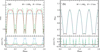 |
Fig. 6. Upper panels: scaled flux as a function of the pulsar phase produced by two antipodal hotspots at the NS surface for two different compactnesses: (a) M = 1.8 M⊙, R = 10 km; (b) M = 1.4 M⊙, R = 13 km. Both the observer inclination and the magnetic obliquity are fixed at 90°. The red solid curves give the results for the exact calculations of bending. Our approximation (given by Eqs. (2) and (17)) is shown with black dotted curves. The blue dashed and green dot-dashed curves correspond to the approximations by Beloborodov (2002) and La Placa et al. (2019), respectively. Lower panels: relative error in the flux for the same three approximations of light bending compared to the exact result. |
4.2. Line profile from an accretion disc
We now consider a problem of line emission from a Keplerian accretion disc around a Schwarzschild BH as discussed, for example, by Chen et al. (1989) and Fabian et al. (1989). We computed the line profile seen by observers at different inclinations i along the direction  . We define a coordinate system with the z-axis being normal to the disc
  , so that the disc lies in the equatorial plane θ = π/2. The radius-vector of the disc surface element at an azimuthal angle φ,
  , makes the angle ψ to the line of sight (see Fig. 7 for geometry):
 (23)
(23)
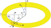 |
Fig. 7. Geometry of emission from an accretion disc ring. |
Because in the Schwarzschild metric, the photon trajectories are planar, the direction of the photon momentum close to the disc surface can be described by a unit vector
![Mathematical equation: $$ \begin{aligned} \hat{\boldsymbol{k}}_0=[ \sin \alpha \ \hat{\boldsymbol{o}} +\sin (\psi -\alpha )\ \hat{\boldsymbol{R}}]/\sin \psi , \end{aligned} $$](/articles/aa/full_html/2020/08/aa37471-20/aa37471-20-eq33.gif) (24)
(24)
where  . The surface element at a (circumferential) radius R is moving with Keplerian velocity v = v(−sin φ, cos φ, 0) with
 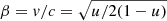 relative to a static observer at this radius (see e.g. Luminet 1979). The corresponding Lorentz factor is
 (25)
(25)
The photon momentum makes angle ξ with the velocity vector
 (26)
(26)
and it makes angle ζ with the local disc normal:
 (27)
(27)
The Doppler factor is
 (28)
(28)
From the Lorentz transformation, one can get the angle that photon momentum makes with the local normal in the comoving frame (see e.g. Poutanen & Gierliński 2003; Poutanen & Beloborodov 2006)
 (29)
(29)
The specific flux observed from a surface element at photon energy E is
 (30)
(30)
where IE is the specific intensity of radiation at infinity, which is related to that in the comoving disc element frame
 (31)
(31)
and the energy ratio (Luminet 1979; Chen et al. 1989)
 (32)
(32)
combines the effects of the gravitational redshift and the Doppler effect. The solid angle occupied by the surface element of area 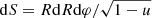 is given by the equation similar to (13):
 (33)
(33)
The observed spectral flux (Eq. (30)) now reads
 (34)
(34)
The observed flux from the disc was then obtained by integrating Eq. (34) over the radius and azimuthal angle
 (35)
(35)
Inside the integrand, for a given R and φ (and given inclination i), we computed ψ using Eq. (23), which was used to get α and 𝒟 using the approach described in Sect. 2. Then ξ and ζ were computed from Eqs. (26) and (27), respectively. Using the Keplerian velocity and the Lorentz factor given by Eq. (25), we then get the Doppler factor δ from Eq. (28). Furthermore, from Eqs. (29) and (32), we get the photon zenith angle in the comoving frame ζ′ and the comoving energy E′, which are needed to obtain  .
.
As an example, we consider a case with isotropic emission in a narrow line centred at comoving energy E0 = 1 with a width of σ = 2 × 10⁻³ from an accretion disc ring extending from 3 to 50 RS with the radial dependence of the emissivity ∝R−2, as was assumed in the original publication by Fabian et al. (1989). The line profiles observed at two inclinations using the exact treatment of light bending and different approximations are shown in Fig. 8. We see that our approximation gives an accuracy better than 0.4%, while other proposed approximations give errors from 1 to 5%. Ignoring the light bending, as was done in the well-known XSPEC (Arnaud 1996) model DISKLINE (Fabian et al. 1989), gives an error that grows from 2% at i = 30° to 20% at i = 60°.
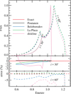 |
Fig. 8. Upper panel: profiles of the emission line from an accretion disc ring extending from 3 to 50 RS around a Schwarzschild BH (or a slowly rotating NS) with the emissivity radial dependence ∝R−2. The solid and dashed curves are for the observer inclination of 30° and 60°, respectively. The red curves correspond to the exact treatment of bending. The results using our new approximation given by Eqs. (2) and (17) are shown with the black curves. The blue and green curves correspond to the approximations of Beloborodov (2002) and La Placa et al. (2019), respectively. All of the curves overlap. The pink curves show the profile with no bending accounted for, as in the XSPEC model DISKLINE. The profiles were re-normalised by a factor giving maximum of unity for the exact profile. Bottom panels: relative error in the line flux for the considered approximations. |
We note that our approximation is nearly independent of the emission radius. For example, if the line is produced in a narrow ring at 3 RS, our approximation gives an accuracy of 0.13% and 1.5% for i = 30° and 60°, respectively, while the corresponding errors are 2.7% and 14% for the Beloborodov (2002) approximations and 1% and 2.8% for the La Placa et al. (2019) approximation. The DISKLINE model, on the other hand, has a typical error of 5% and 15%, respectively, but it rises sharply towards the line peaks and reaches 40% and 70% there.
Wilkins & Fabian (2011) show that the line profiles from accretion discs mostly depend on the inner disc radius, which is the function of the black hole spin, while the effect of the spin on photon trajectories is minor. Because our approximation works equally well for emission radii that are well within 3 RS (see Fig. 5), it can, in principle, be used for calculations of the line profiles from the discs around rotating black holes too. Detailed calculations are left for future work.
5. Summary
In this paper, we propose a new approximation for light bending in the Schwarzschild metric. It can be applied to any emission point above the horizon of a BH and also for trajectories that pass through the turning point, but which make less than half of a full turn. For emission radii above the photon orbit at the 1.5 Schwarzschild radius, the approximation has an accuracy of better than 0.2% for the bending angle and 3% for the lensing factor for photon orbits turning by less than 160° around a compact object. This approximation can be useful for problems involving rotating oblate NSs and an accretion disc around a compact object when fast accurate calculations of light bending are required. The proposed formulae can also be used to check the results of exact calculations.
A similar approach for the lensing factor was used by De Falco et al. (2016). That paper, however, has a number of flaws, for example, calculations of the bending angle for α > π/2 assumed ψmax = ψ(R, α = π/2) instead of the correct ψmax = ψ(p, α = π/2), see Eq. (11); the expression for the solid angle, which is proportional to our lensing factor, contains an excessive factor sin α/sin ψ; there is an error in Eq. (30), where 1 − C… should be −1/2 − C… instead; and the pulse profiles from a hotspot on a rapidly rotating NS in their Fig. 9 have unphysical jumps before eclipses, instead of going to zero.
Acknowledgments
This research has been supported by the grant 14.W03.31.0021 of the Ministry of Science and Higher Education of the Russian Federation and the Academy of Finland grants 322779 and 333112. I thank Joonas Nättilä and Dmitry Yakovlev for comments.
References
- Arnaud, K. A. 1996, in Astronomical Data Analysis Software and Systems V, eds. G. H. Jacoby, & J. Barnes (San Francisco: ASP), ASP Conf. Ser., 101, 17 [Google Scholar]
- Beloborodov, A. M. 2002, ApJ, 566, L85 [NASA ADS] [CrossRef] [Google Scholar]
- Bogdanov, S., Lamb, F. K., Mahmoodifar, S., et al. 2019, ApJ, 887, L26 [CrossRef] [Google Scholar]
- Chen, K., Halpern, J. P., & Filippenko, A. V. 1989, ApJ, 339, 742 [NASA ADS] [CrossRef] [Google Scholar]
- De Falco, V., Falanga, M., & Stella, L. 2016, A&A, 595, A38 [NASA ADS] [CrossRef] [EDP Sciences] [Google Scholar]
- Dexter, J. 2016, MNRAS, 462, 115 [NASA ADS] [CrossRef] [Google Scholar]
- Fabian, A. C., Rees, M. J., Stella, L., & White, N. E. 1989, MNRAS, 238, 729 [NASA ADS] [CrossRef] [Google Scholar]
- La Placa, R., Bakala, P., Stella, L., & Falanga, M. 2019, Res. Notes Am. Astron. Soc., 3, 99 [CrossRef] [Google Scholar]
- Luminet, J. P. 1979, A&A, 75, 228 [Google Scholar]
- Miller, M. C., & Lamb, F. K. 2015, ApJ, 808, 31 [NASA ADS] [CrossRef] [Google Scholar]
- Miller, M. C., Lamb, F. K., Dittmann, A. J., et al. 2019, ApJ, 887, L24 [Google Scholar]
- Misner, C. W., Thorne, K. S., & Wheeler, J. A. 1973, Gravitation (San Francisco: W. H. Freeman and Co.) [Google Scholar]
- Nättilä, J., & Pihajoki, P. 2018, A&A, 615, A50 [NASA ADS] [CrossRef] [EDP Sciences] [Google Scholar]
- Pechenick, K. R., Ftaclas, C., & Cohen, J. M. 1983, ApJ, 274, 846 [NASA ADS] [CrossRef] [Google Scholar]
- Poutanen, J., & Beloborodov, A. M. 2006, MNRAS, 373, 836 [NASA ADS] [CrossRef] [Google Scholar]
- Poutanen, J., & Gierliński, M. 2003, MNRAS, 343, 1301 [NASA ADS] [CrossRef] [Google Scholar]
- Riley, T. E., Watts, A. L., Bogdanov, S., et al. 2019, ApJ, 887, L21 [NASA ADS] [CrossRef] [Google Scholar]
- Salmi, T., Nättilä, J., & Poutanen, J. 2018, A&A, 618, A161 [NASA ADS] [CrossRef] [EDP Sciences] [Google Scholar]
- Semerák, O. 2015, ApJ, 800, 77 [CrossRef] [Google Scholar]
- Watts, A. L., Andersson, N., Chakrabarty, D., et al. 2016, Rev. Mod. Phys., 88, 021001 [NASA ADS] [CrossRef] [Google Scholar]
- Wilkins, D. R., & Fabian, A. C. 2011, MNRAS, 414, 1269 [NASA ADS] [CrossRef] [Google Scholar]
All Figures
|
Fig. 1. Geometry of light bending in the Schwarzschild metric. The observer is situated on the right at ψ = 0. |
| In the text | |
|
Fig. 2. Light bending relation between the cosine of the emission angle α and the angle ψ between the line of sight and the radius-vector of the emission point computed using exact relations (6)–(11) for the Schwarzschild metric for six different emission radii R/RS = 1.1, 1.3, 1.5, 2, 3, and 10, which are marked next to the corresponding curves. |
| In the text | |
|
Fig. 3. Upper panel: light bending relation between the cosine of the emission angle α and the cosine of the angle ψ between the line of sight and the radius-vector of the emission point in the Schwarzschild metric. The red curves give the exact relation. Our new approximate relation (2) is shown with the black curves. The blue straight lines are for the Beloborodov (2002) approximation (1), while the green curves represent the approximation (16) by La Placa et al. (2019). The red, green, and black curves practically coincide. The solid, dotted, dashed, and dot-dashed curves correspond to radii R/RS = 1.5, 2, 2.5, and 3, respectively. Bottom panel: relative error of the emission angle δα/α for three approximations as compared to the exact result. Same notations as in the upper panel. |
| In the text | |
|
Fig. 4. Same as Fig. 3, but for the lensing factor 𝒟. The approximation (20) is shown by the pink curves. |
| In the text | |
|
Fig. 5. Contours of the constant relative error on (a) the bending angle δα/α and (b) the lensing factor for our approximations given by Eqs. (2) and (17). Neighbouring contours differ by a factor of 10 in the value of the error. Solid and dotted curves represent positive and negative deviations, respectively. |
| In the text | |
|
Fig. 6. Upper panels: scaled flux as a function of the pulsar phase produced by two antipodal hotspots at the NS surface for two different compactnesses: (a) M = 1.8 M⊙, R = 10 km; (b) M = 1.4 M⊙, R = 13 km. Both the observer inclination and the magnetic obliquity are fixed at 90°. The red solid curves give the results for the exact calculations of bending. Our approximation (given by Eqs. (2) and (17)) is shown with black dotted curves. The blue dashed and green dot-dashed curves correspond to the approximations by Beloborodov (2002) and La Placa et al. (2019), respectively. Lower panels: relative error in the flux for the same three approximations of light bending compared to the exact result. |
| In the text | |
|
Fig. 7. Geometry of emission from an accretion disc ring. |
| In the text | |
|
Fig. 8. Upper panel: profiles of the emission line from an accretion disc ring extending from 3 to 50 RS around a Schwarzschild BH (or a slowly rotating NS) with the emissivity radial dependence ∝R−2. The solid and dashed curves are for the observer inclination of 30° and 60°, respectively. The red curves correspond to the exact treatment of bending. The results using our new approximation given by Eqs. (2) and (17) are shown with the black curves. The blue and green curves correspond to the approximations of Beloborodov (2002) and La Placa et al. (2019), respectively. All of the curves overlap. The pink curves show the profile with no bending accounted for, as in the XSPEC model DISKLINE. The profiles were re-normalised by a factor giving maximum of unity for the exact profile. Bottom panels: relative error in the line flux for the considered approximations. |
| In the text | |
Current usage metrics show cumulative count of Article Views (full-text article views including HTML views, PDF and ePub downloads, according to the available data) and Abstracts Views on Vision4Press platform.
Data correspond to usage on the plateform after 2015. The current usage metrics is available 48-96 hours after online publication and is updated daily on week days.
Initial download of the metrics may take a while.