| Issue |
A&A
Volume 634, February 2020
|
|
|---|---|---|
| Article Number | A66 | |
| Number of page(s) | 14 | |
| Section | Galactic structure, stellar clusters and populations | |
| DOI | https://doi.org/10.1051/0004-6361/201936711 | |
| Published online | 10 February 2020 | |
Gaia-DR2 extended kinematical maps
II. Dynamics in the Galactic disk explaining radial and vertical velocities
1
Instituto de Astrofísica de Canarias, 38205 La Laguna, Tenerife, Spain
e-mail: This email address is being protected from spambots. You need JavaScript enabled to view it.
2
Departamento de Astrofísica, Universidad de La Laguna, 38206 La Laguna, Tenerife, Spain
3
South–Western Institute for Astronomy Research, Yunnan University, Kunming 650500, PR China
4
Department of Astronomy, China West Normal University, Nanchong 637009, PR China
5
Museo Storico della Fisica e Centro Studi e Ricerche Enrico Fermi, Compendio del Viminale, 00184 Rome, Italy
6
Istituto dei Sistemi Complessi, Consiglio Nazionale delle Ricerche, 00185 Roma, Italy
7
Istituto Nazionale Fisica Nucleare, Unità Roma 1, Dipartimento di Fisica, Universitá di Roma “Sapienza”, 00185 Roma, Italy
8
Faculty of Mathematics, Physics, and Informatics, Comenius University, Mlynska dolina, 842 48 Bratislava, Slovakia
9
Key Laboratory of Optical Astronomy, National Astronomical Observatories, Chinese Academy of Sciences, Beijing 100012, PR China
10
Purple Mountain Observatory, the Partner Group of MPI für Astronomie, 2 West Beijing Road, Nanjing 210008, PR China
11
Nordic Institute of Theoretical Physics, Roslagstullsbacken 23, 106 91 Stockholm, Sweden
Received:
16
September
2019
Accepted:
21
December
2019
Abstract
Context. In our Paper I, by using statistical deconvolution methods, extended kinematics maps of Gaia-DR2 data have been produced in a range of heliocentric distances that are a factor of two to three larger than those analyzed previously by the Gaia Collaboration with the same data. It added the range of Galactocentric distances between 13 kpc and 20 kpc to the previous maps.
Aims. Here, we investigate the dynamical effects produced by different mechanisms that can explain the radial and vertical components of these extended kinematic maps, including a decomposition of bending and breathing of the vertical components. This paper as a whole tries to be a compendium of different dynamical mechanisms whose predictions can be compared to the kinematic maps.
Methods. Using analytical methods or simulations, we are able to predict the main dynamical factors and compare them to the predictions of the extended kinematic maps of Gaia-DR2.
Results. The gravitational influence of Galactic components that are different from the disk, such as the long bar or bulge, the spiral arms, or a tidal interaction with Sagittarius dwarf galaxy, may explain some features of the velocity maps, especially in the inner parts of the disk. However, they are not sufficient in explaining the most conspicuous gradients in the outer disk. Vertical motions might be dominated by external perturbations or mergers, although a minor component may be due to a warp whose amplitude evolves with time. Here, we show with two different methods, which analyze the dispersion of velocities, that the mass distribution of the disk is flared. Despite these partial explanations, the main observed features can only be explained in terms of out-of-equilibrium models, which are either due to external perturbers or to the fact that the disk has not had time to reach equilibrium since its formation.
Key words: Galaxy: kinematics and dynamics / Galaxy: disk
LAMOST fellow.
© ESO 2020
1. Introduction
The connection between kinematics and dynamics has been intensively studied during the last decades of research about the Milky Way as a Galaxy (Binney & Tremaine 2008). Different sources of spectroscopic data have been used to obtain information about the forces that dominate the Galactic motions; for instance, with Sloan Digital Sky Survey (SDSS; Moni Bidin et al. 2012), Apache Point Observatory Galactic Evolution Experiment (APOGEE; Bovy et al. 2014), and Radial Velocity Experiment (RAVE; Binney et al. 2014) surveys. However, the important moment pertaining to the major exploitation of six-dimensional (6D) phase space (3D spatial and 3D velocity) maps occurred thanks to the kinematic maps of Gaia data Gaia Collaboration (2018, hereafter GC18); the disk being the component with better analysis prospects due to the low distance and extinction of the sources around the Sun and toward the anticenter. The analysis by GC18 of Gaia-DR2 has provided kinematical maps for Galactocentric distances of R < 13 kpc. Carrillo et al. (2019), assuming priors about the stellar distribution, slightly extended the mapping out to R = 14 − 16 kpc for these kinematic maps. By using the Large Sky Area Multi-Object Fibre Spectroscopic Telescope (LAMOST) or the LAMOST and Gaia surveys, other three-dimensional (3D) kinematical maps covering a similar range of Galactocentric distances were obtained (Wang et al. 2018a, 2019, 2020).
In López-Corredoira & Sylos Labini (2019, hereafter Paper I), the kinematics maps of Gaia-DR2 data were extended in a range of heliocentric distances by a factor of two to three larger with respect to GC18, out to R = 20 kpc, by applying a statistical deconvolution of the parallax errors based on the Lucy’s inversion method of the Fredholm integral equations of the first kind. This extension to farther distances is interesting for the kinematical studies of the disk because many relevant features, aside from an axisymmetric disk in equilibrium, occur at R > 13 kpc. The warp, flare, and most significant fluctuations with respect to zero radial or vertical velocities, take place where the density of the disk is lower, so it is worth extending the analysis beyond 13 kpc from the Galactic center. The newly extended maps provide substantial, new and corroborated information about the disk kinematics pertaining to the following: significant departures from circularity in the mean orbits with radial Galactocentric velocities between −20 and +20 km s−1 and vertical velocities between −10 and +10 km s−1; variations of the azimuthal velocity with position; asymmetries between the northern and the southern Galactic hemispheres, especially toward the anticenter that includes a larger azimuthal velocity in the south; and others. This shows us that the Milky Way (MW) is far from a simple stationary configuration in rotational equilibrium, but it is characterized by streaming motions in all velocity components with conspicuous velocity gradients.
In the present paper, we investigate the dynamical effects produced by different physical mechanisms that can explain the kinematic maps derived in Paper I. The paper is organized as follows: in Sects. 2.1 and 2.2, we describe the main features of the radial and vertical velocities obtained in Paper I. A decomposition of bending and breathing of the vertical components (i.e., the mean and the difference of the median vertical velocities in symmetric layers with respect to the Galactic mid-plane) is given in Sect. 3. An analysis of the azimuthal velocities and the derivation of the rotation speed will be treated in another paper (Chrobàková et al., in prep., Paper III). In the following sections, we explore whether already known morphological features of the Galactic disk can explain, at least in part, the observed trends in the radial and vertical velocities. In Sect. 4, we analyze the effect of the Galactic bar both in the inner and the outer disk regions. In Sect. 5, we explore the gravitational effects produced by the overdensities associated to the spiral arms. In Sect. 6, the kinematical consequences, especially in vertical velocities of minor mergers or the interaction with satellites, is explored with the help of some N-body simulations. The distortions of the disk and their effect over the median velocities and their dispersion due to the warp or the flare are studied in Sects. 7 and 8 respectively. Finally, an interpretation of the observed kinematical features in terms of out-of-equilibrium (Sect. 9) seems to give a possible framework for the non-null radial and vertical velocities; in this picture, the transient nature of the outer part of the disk and of the arms is related to the presence of coherent radial velocities, with both negative (i.e., contraction) and positive (i.e., expansion) signs. Discussions and conclusions are given in the last section. The paper as a whole tries to be a compendium of dynamical factors that can be tested through the direct observable variables: the kinematic maps. Rather than a bibliographic review, the paper acts as more so a general reflection within the wide topic of the forces acting in the disk of our Galaxy through the application of the different hypotheses to our extended kinematic maps of Gaia-DR2.
2. Vertical and radial asymmetrical motions in Paper I
2.1. Radial Galactocentric velocities
One of the main results of Paper I is that the radial component of the velocity displays considerable gradients. In particular, the top of Fig. 8 in Paper I shows significant radial Galactocentric velocities (VR) between −20 and +20 km s−1. Previous analyses in the direction of the anticenter (López-Corredoira & González-Fernández 2016; Tian et al. 2017; López-Corredoira et al. 2019) have already shown these departures of mean circular orbits. However, the analysis of Paper I has furthermore provided the azimuthal dependence of the radial velocity component, which allows one to better compare it with some possible physical scenarios. An average ellipticity or lopsidedness may be present in the highest R disk (López-Corredoira & González-Fernández 2016; López-Corredoira et al. 2019). Also, a secular expansion and contraction of the disk (López-Corredoira & González-Fernández 2016; López-Corredoira et al. 2019) cannot be independent of the azimuth, but it may affect some parts of the disk; as we see in the top left corner of Fig. 8 of Paper I, the expansion and contraction affect different parts of the disk differently: we see expansion (VR > 0) for azimuths −5° ≲ϕ ≲ 60° and R > 10 kpc, whereas there is contraction (VR < 0) for azimuths −50° ≲ϕ ≲ −5° and R > 10 kpc. Only within |ϕ|≲25° do we have errors that are lower than 10 km s−1, which makes the detection significant.
We note that the effect of a zero-point systematic error in parallaxes has already been evaluated (Paper I, Sect. 4.4). Figure 16 of Paper I shows the velocity maps with the most likely value of zero-point shift in parallaxes of −0.03 mas. and the gradients changed very slightly with respect to nonzero-point-correction. On the top of Fig. 1, we reproduce the radial velocity maps with a zoom on the region within |Y| < 8 kpc. We also note that the gradients and the change of sign of VR is observed near the anticenter area (not exactly in the change of quadrant though), where VR is almost only dependent on radial heliocentric velocities and its sign would be rather insensitive to the distance determination. In any case, the propagation of errors of Δr was taken into account, so the effect of systematic errors in the parallaxes should not be dominant. Furthermore and as previously mentioned, in the anticenter, the radial velocities were demonstrated to reach values up to 20 km s−1 in absolute value with data that is different from Gaia (López-Corredoira et al. 2019).
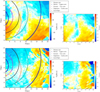 |
Fig. 1. Left: Gaia extended kinematic maps (Fig. 8 of Paper I) with the over-plotting of the representation of the spiral arms: four main spiral arms follow the model of Vallée (2017) and the local spur modeled by Hou & Han (2014): upper panel, radial velocity; bottom panel, vertical velocity. Right: Gaia extended kinematic maps introducing a correction to the zero-point bias of parallaxes πc = π + 0.03 mas (Fig. 16 of Paper I). |
Large scale motions corresponding to expansion and contraction in different parts of the outer disk are taking place, suggesting that giant processes of inflows and outflows of stars are occurring in our Galaxy. The ratio of mass exchange in these flows may be estimated with a density model of the disk together with the information of the velocities. By assuming the extension of the flow of Δϕ = 40° and by using the method introduced by López-Corredoira et al. (2019, Sect. 4.2), we get mass accretion and ejection of ∼5 × 10⁸ M⊙ Gyr−1 either inwards or outwards.
2.2. Vertical Galactocentric velocities
The maps of vertical velocity component shown in Paper I are complex and their physical explanation has to be found in combining a variety of events. Nonaxisymmetric features have been seen previously in the kinematics of the Milky Way (Faure et al. 2014; Bovy et al. 2015), showing a velocity distribution in the Galactic disk that is not smooth. With the use of the data from the Gaia mission (GC18, Paper I), it is now possible to extend these analyses outside the Solar vicinity with more statistical significance. The observed velocities between −10 and +10 km s−1 with some correlated gradients require the existence of some vertical forces in the Galactic dynamics. On the bottom of Fig. 1, we reproduce the radial velocity maps with a zoom on the region within |Y| < 8 kpc; the zero-point-correction of parallaxes is not important.
3. Bending and breathing for vertical motions of the Galactic disk
Bending and breathing modes in the galactic disk have been discussed in Weinberg (1991) as a measure of vertical oscillations of the Galactic disk. We have used the data in Paper I to compute the bending and breathing vertical velocities at several heights over the disk, following the definitions for breathing and bending velocities in GC18 (see the paper for details):
![Mathematical equation: $$ \begin{aligned} V_{\rm bending}(X,Y;Z)=\frac{1}{2}[V_Z(X,Y,Z)+V_Z(X,Y,-Z)] \end{aligned} $$](/articles/aa/full_html/2020/02/aa36711-19/aa36711-19-eq1.gif) (1)
(1)
and
![Mathematical equation: $$ \begin{aligned} V_{\rm breathing}(X,Y;Z)=\frac{1}{2}[V_Z(X,Y,Z)-V_Z(X,Y,-Z)] ,\end{aligned} $$](/articles/aa/full_html/2020/02/aa36711-19/aa36711-19-eq2.gif) (2)
(2)
while our analysis is extended much further away than the velocity analysis from the Solar vicinity. In Fig. 2, we plot the results of the analysis following the same graphical layout of GC18 for comparison purposes. The reader must be aware that the definition of the X coordinate is different in this paper than in GC18. In both works, the Galactic center is at X = 0, while the Sun is at X = 8.34 kpc in this paper and in X = −8.34 kpc in GC18. Both Fig. 2 here and Fig. C6 in GC18 are centered around the Sun projection in the Galactic plane. The data have been binned in cells of 400 × 400 pc in XY, which are then averaged in layers of 400 pc in Z that are above and below the plane, in order to produce the final bending and breathing distribution. The right column panels in Fig. 2 shows the root-mean-square (r.m.s.) errors in the velocities. The bending velocity is negative in the inner disk, reaching values in excess of −5 km s−1, while it is increasingly positive in the outer disk and the height of the layers are above and below the plane, with peaks over 5 km s−1. The breathing velocity shows a smoother distribution, which is mostly negligible in the plane, predominantly positive in the second and fourth quadrants of Fig. 2, and negative in the first one. The third quadrant shows a mixture of both negative and positive values. This distribution is more marked when it is far from the plane.
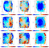 |
Fig. 2. Bending and breathing velocities, using the same graphic layout and panel distribution as in GC18. Left column panels: bending vertical velocity; middle column panels: breathing vertical velocities; and right column panels: error in the computed values for both bending and breathing modes. Units of velocities in km s−1; units of scale X, Y in kpc. Position of the Sun at X = 8.34, Y = 0; position of the Galactic center at X = 0, Y = 0. See text. |
In recent years, several papers have been devoted to exploring vertical motions in the Galaxy. Widrow et al. (2012) claim, based on the analysis of 11 000 stars in Sloan Extension for Galactic Understanding and Exploration (SDSS-SEGUE), that the motion of stars resemble that of a breathing mode perturbation with a velocity gradient of ∼3 − 5 km s−1 kpc−1. That would result in a negative bending velocity distribution, which is more negative with the distance off the plane and a positive breathing velocity distribution. This was more marked before with the distance off the plane. This is not supported by the data in Fig. 2. Widrow et al. (2012) also show an increase of the velocity dispersion with the distance off the plane, which is attributed to a progressively larger number of kinematically hot stars from the thick disk. We show in Sect. 8 that the flaring of the Galactic disk can explain this, at least to a certain level.
More recently, Carrillo et al. (2018) computed 3D velocities of a large sample of Galactic sources using radial velocities from RAVE, astrometric solution from the Tycho-Gaia Astrometric Solution (TGAS) and proper motions from several catalogs. They find differences in the velocity distributions derived from each of the proper motion data bases, which display combinations of bending and breathing modes. Our results seem to be aligned with their claim (see also Carrillo et al. 2019; Bennett & Bovy 2019) of having detected a breathing mode inside the solar circle, which would correspond to positive breathing velocity in the second and third quadrant of Fig. 2, and a bending mode outside it, which would yield to a positive bending velocity in the first and fourth quadrants. However, in agreement with Bennett & Bovy (2019), we see clear asymmetry in the vertical velocity above and below the plane as the bending and breathing velocities do not follow antisymmetric patterns. The interior of the breathing mode to the solar circle is more marked in the negative values of the bending velocity distribution than in the corresponding positive values of the breathing velocity in the same area. This difference is more noticeable closer to the plane. Additionally, the same thing seems to happen for the bending mode beyond the Sun; the bending velocity distribution shows a more clear positive average value than the breathing velocity distribution does with its positive value. However, due the complex nature of the observed vertical velocity distribution, it is difficult to make a reasonable description by only using a single oscillation mode. As noted in GC18, a superposition of different modes is likely to be the true distribution.
4. The effect of the Galactic bar on the radial velocities of stars in the Galactic disk
In recent years, several papers have investigated the effect of the central region of the Milky Way Galaxy on the radial mixing of the Galactic disk and radial migration of stars. In this section, we intend to compare the observed features provided by kinematical maps of Paper I with results of published numerical simulations. Halle et al. (2018) present a complex N-body simulation of the Galactic disk by focusing on the radial migration of stars. The model considers the Galactic bar as the strongest nonaxisymmetrical perturbation, whose angular speed decreases due to the transfer of angular momentum from the disk to the dark matter halo. The consequence of the slowing Galactic bar is an outwards-shifting of the corotation radius, thus it implies that a wider range of the Galactocentric distances is affected by the corotating resonance. The thin disk stars significantly migrate outwards near the corotating radius at approximately 10 kpc. In the case of the thick disk, the average initial radius of stars, which is influenced by the corotation resonance, is slightly shifted to lower Galactocentric distances (Halle et al. 2018). This result is in accordance with the top panel of Fig. 2 in Paper I. However, the complex behavior of radial velocities that are plotted in the top panel of Figs. 8 and 13 of Paper I cannot simply be explained by the simulations by Halle et al. (2018). One can also compare the dependence of the dispersion of the radial velocities on the Galactocentric distance (Fig. A2 Halle et al. 2018) with the observational data. We can say that the closest fit to the observed radial velocity dispersion represents the thick disk model by Halle et al. (2018), but there is no evidence that the model that was used for the Galactic bar could generate observed dispersion of radial velocities.
Monari et al. (2014) tested different structural parameters of the Galactic bar, but they all had a constant pattern speed of Ωb = 50 km s−1 kpc−1. They consider a default bar to be a long bar and a less massive bar. The simulation covers the region around the Sun (approximately from 6 kpc to 9 kpc); the dependence of the radial velocity on the Galactocentric distance for different Z in the center-Sun-anticenter direction and for various bar models is plotted (Figs. 4–8 of Monari et al. 2014). All the results of Monari et al. (2014) show the same trend, which is a decrease in the radial velocities from positive to negative values with increasing Galactocentric distances in the vicinity of the Sun. However, the behavior of the radial velocities observed in Paper I, which are plotted in Fig. 3, is more complex. By comparing the red line of Fig. 3 (−0.25 kpc < z < +0.25 kpc) with the results of Monari et al. (2014) in the considered range of Galactocentric distances, we see that the simulations cannot explain the observed features. Only for the specific range of 0.5 kpc < z < +1.0 kpc, the results of Monari et al. (2014) are similar to the observations (refer to the blue line in Fig. 3 with the rightmost panel of Fig. 7 in Monari et al. 2014). Carrillo et al. (2019) also investigate the kinematics of the Galaxy by using the second data release of the Gaia mission (GC18). In the X − Y plane, they observed an asymmetry in the radial velocities; a positive sign of the radial velocity in the first quadrant and a negative sign in the quadrant for X ≲ 5 kpc. The same feature can also be observed in Fig. 8 of Paper I and it is clearly visible in Fig. 4 of the present paper for various values of X. Carrillo et al. (2019) try to explain the pattern as a result of the presence of the Galactic bar. They could not reproduce the observed azimuthal gradient when just considering internal effects (e.g., the Galactic bar and the spiral arms).
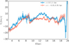 |
Fig. 3. Mean value of radial velocity over various z intervals as a function of the Galactocentric distance along the center-Sun-anticenter direction using data by Paper I. |
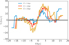 |
Fig. 4. Mean value of radial velocity as a function of Y for various values of X by using data from Paper I. |
We have also investigated the evolution of radial velocities by using the results of integration of 105 test particles randomly distributed in the Galactic equatorial plane in the rotating gravitational potential of the Galactic bar (Ωbar = 55.5 km s−1 kpc−1, Mbar = 9.23 × 10⁹ M⊙) that were obtained by Kačala et al. (2018). The simulation considered two approaches, the first one is based on the Newtonian gravitation including the Navarro-Frenk-White (NFW) dark matter halo (Navarro et al. 1997), the second one uses non-Newtonian gravitation (Modified Newtonian Dynamics; MOND) based on McGaugh et al. (2016) without a dark matter halo that takes the following equation of motion into account (Kačala et al. 2018):
 (3)
(3)
where g+ = 1.2 × 10⁻¹⁰ m s−2, Φb is the gravitational potential of the Galactic bar, and Φd is the gravitational of the Galactic disk. The results of the simulations (see Figs. 5 and 6) cannot account for the observed behavior of the radial velocities seen in Fig. 8 of Paper I (a positive and negative sign of the radial velocity for X ≳ 10 kpc and azimuths −5° ≲ϕ ≲ 60° and −50° ≲ϕ ≲ −5°, respectively). The simulations give average values of the fluctuations, which are much lower than the observed ones, and fastly varying fluctuations, which are not observed in the smooth gradient of our data. Thus, we cannot conclude that the observed feature is caused by the effect of the Galactic bar.
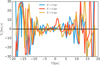 |
Fig. 5. Mean value of radial velocity as a function of Y for various values of X by using results of integration of 105 test particles in the rotating gravitational potential of the Galactic bar considering Newtonian dynamics. |
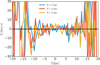 |
Fig. 6. Mean value of radial velocity as a function of Y for various values of X by using results of integration of 105 test particles in the rotating gravitational potential of the Galactic bar considering MOND. |
5. Spiral arms
When spiral arms pull stars toward them, they may generate peculiar acceleration. This mechanism, with compression where the stars enter the spiral arm and expansion where they exit, was proposed as a tentative explanation for the variations of more local radial velocities (Siebert et al. 2011; Monari et al. 2016; Gaia Collaboration 2018; López-Corredoira et al. 2019); furthermore, some ripples and ridges in the kinematics may be formed due to the spiral arms (Faure et al. 2014; Hunt et al. 2018; Quillen et al. 2018). A galaxy with four spiral arms with a total mass of ∼3 × 10⁹ M⊙ (∼3% of the Galactic disk mass) would give radial galactocentric velocities with an amplitude of ∼6 km s−1 (López-Corredoira et al. 2019), which might be part of the explanation of the observed VR.
Figure 6 of Faure et al. (2014) shows that the transition when crossing a spiral arm from positive to negative velocities (or vice verse) is smooth when within short distances, and the value of ⟨VR⟩ is expected to be quite stable in the inter-arm region. From this figure, we also see that the map of VR changes should follow the pattern of the spiral arms. A similar pattern is also obtained in a scenario of out-of-equilibrium formation of disk and spiral arms (see Sect. 9), as observed in Fig. 14 of López-Corredoira et al. (2019). The question is inevitably posed as to whether this is observed in our Gaia data. Figure 1 shows the Gaia extended kinematic maps (Fig. 8 of Paper I) with the over-plotting of the representation of the following spiral arms: four main spiral arms following the model of Vallée (2017) and the local spur modeled by Hou & Han (2014).
In the radial velocity plot, we see some possible coincidences of zero speed tracing some spiral arms, such as Scutum-Crux, local spur, or Perseus. However, some zones of transition between positive and negative velocities, such as the most prominent one between (X = 10, Y = −5) and (X = 18, Y = 0) (units in kpc) with a radial velocity gradient between these two regions of about 40 km s−1, clearly cannot trace any spiral arms; indeed, this line is perpendicular to the known spiral arms. For the vertical velocity map, we do not see any clear association at all between spiral arms and the observed features. Therefore, we conjecture that spiral arms can only be a partial explanation for the radial velocities, and some other effect should produce main features with higher amplitudes than expected from spiral arms (∼6 km s−1) and with a different distribution. In particular, the large scale motions of expansion and contraction in different parts of the outer disk at R ≳ 10 kpc with giant processes of inflows and outflows of stars are not due to the spiral arms.
6. Minor mergers and interaction with satellites
Carrillo et al. (2019) propose that a major perturbation, such as the impact of the Sagittarius dwarf galaxy, could reproduce the observed VR field. Incorporating an impact of a dwarf galaxy as an external perturbation matches the observed velocity fields. Carrillo et al. (2019) conclude that the azimuthal radial velocity gradient is strongly time-dependent and the radial velocity field will reverse after the effect of the external perturbation vanishes. There are some indications (Fig. 10 of Carrillo et al. 2019) that the merger could cause another interesting feature in the radial velocity profile, such as the change of sign of the radial velocity as observed in Paper I. The comparison of the result of the simulation (Fig. 10 of Carrillo et al. 2019) with the observed pattern of Paper I is not conclusive, we see some similar features but also some relevant differences.
Another perspective is given by Tian et al. (2017), who claim that it is not likely that the perturbations produced by mergers may intensively affect the in-plane velocity. Also, a local stream cannot be the explanation for radial velocities along a wide range of ∼20 kpc, but it could be a large-scale stream associated with the Galaxy in the Sun–Galactic center line. We do not have evidence for such a huge structure embedded in our Galaxy, so we think this is not very likely. Moreover, there is a very small asymmetry of radial velocities between the northern and southern Galactic hemispheres (Figs. 9–12/top left of Paper I), thus we think it is very unlikely that the same stream that is independent of the Galaxy be so symmetric with respect to the plane.
Nonetheless, minor mergers may raise vertical waves (Gómez et al. 2013). Major mergers (1:10) along the history of the Milky Way are excluded from chemodynamical analyses (Ruchti et al. 2014, 2015). Also, Haines et al. (2019) explore the effect of the passage of a massive satellite through the disk of a spiral galaxy and, in particular, the induced vertical wobbles in a time varying potential.
Here, we use a static analytic potential to model the dark matter halo of the MW, while particles are used to model stars in the disk and the bulge. For satellites, particles are used for both dark matter and stars. We modeled the accretion of nine satellites that infall in the first 0−4 Gyr. The dark matter halo of the MW is described as an NFW potential (Navarro et al. 1997) with a virial mass of Mvir = 1 × 10¹² M⊙ and a concentration parameter of c = 7 (Macciò et al. 2008). The stellar part of the MW is 3% of the virial mass (Moster et al. 2013; Wang et al. 2015), consisting of a Hernquist bulge (Hernquist 1990) and an exponential disk. The bulge contributes 20% of the total stellar mass, and the remaining 80% of the total stellar mass is in the disk. Our dynamical model is simple, we just want to investigate qualitatively how multiple minor mergers affect the asymmetry of the disk of the Milky Way and discuss the possible mechanisms of these asymmetries, so the accuracy of the parameters is not important here. We designed three types of progenitors: H-m, M-m, and L-m, with total masses of 4 × 10¹⁰ M⊙, 1 × 10¹⁰ M⊙, and 2.5 × 10⁹ M⊙, respectively. Using H-m, M-m, and L-m, we created nine satellites (three for each) with distinct infall scenarios by changing their initial velocities and positions. Each satellite has an NFW dark matter halo and an exponential stellar disk. The total simulation time is 12 Gyr, then we selected all the particles with a radius from 8 to 20 kpc, a height from −2 to 2 kpc, and the stars are located in a sector of 15 degree azimuth. For more details about orbit parameters, see Yuan et al. (2018).
Figure 7 shows edge−on views of the kinematics of the disk with a range of 8.5−17.5 kpc, which is shown as median velocity maps of VZ (in km−1). There are general vertical bulk motions or bending mode motions in the range of 10−17 kpc with few negative value bins. For the distance that is less than 10 kpc, there are some bins with a negative or zero value; it is matched to the general trend with Fig. 10 of Paper I by considering observational errors. The pattern of the vertical motions larger than 9 kpc is similar to other works using LAMOST survey (Wang et al. 2018a, 2019, 2020) for the overall trend. Here we have just chosen one snapshot to investigate the effects occurring on the disk when some or many satellites interact with the galaxy. The results show that it can reconstruct recent Gaia kinematical features in some parts of the disk. Other angles are shown in Fig. 8. It is important to note, however, that there is no evidence of the existence of so many minor mergers in the Milky Way.
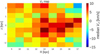 |
Fig. 7. Edge−on views of the kinematics of the disk with range of 8.5−17.5 kpc, shown as median velocity maps of VZ (in km−1) in the N-body simulation. There are clear vertical bulk motions or bending mode motions in the range of 10−17 kpc; especially for Z when less than 2 kpc. |
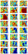 |
Fig. 8. Edge−on views of the kinematics of the disk with range of R = 8–20 kpc and Z = −2.5–2.5 kpc, shown as median velocity maps of VZ (in km−1) for different azimuthal angles in the N-body simulation. Colors and labels are the same as in Fig. 7. |
7. The Galactic warp
Warps are common phenomena in disk galaxies (Bosma 1991) that have been a well known feature of the Milky Way disk for a long time, which was both observed in the gas and in the stellar components (and references therein Miyamoto et al. 1993; Miyamoto & Zhu 1998; Drimmel et al. 2000; López-Corredoira et al. 2002a; Reylé et al. 2009). At present, there are several scenarios as to the origin and evolution of the Galactic warp (Castro-Rodríguez et al. 2002): interactions with the dark matter halo or nearby galaxies, infall, or others. Transient or long-lived features and some clues about its nature can be derived by using the detailed kinematics emerging from the Gaia data. Huang et al. (2018), Poggio et al. (2018), Wang et al. (2019) and Romero-Gómez et al. (2019) have already shown kinematical signatures of the Galactic warp with Gaia and other data, and here we continue such analyses within farther Galactocentric distances.
To this end, we used the warp model in López-Corredoira et al. (2014) to fit the vertical velocity (Vz) distribution with the Galactic azimuth presented in Paper I (see its Fig. 15). We selected the data at Galactocentric of radii 12 kpc and 16 kpc. The data were fit to the model prediction for the vertical velocity, which include two terms for the vertical velocity; a first one for the inclination of the orbits and the second from the temporal variation of the amplitude of the warp:
![Mathematical equation: $$ \begin{aligned} \mathrm{Max}[Z_{\rm warp}]=\gamma (R-R_\odot )^\alpha ,\end{aligned} $$](/articles/aa/full_html/2020/02/aa36711-19/aa36711-19-eq4.gif) (4)
(4)
![Mathematical equation: $$ \begin{aligned} V_{\rm Z}(R > {R_ \odot },\phi ,z = 0) =&\frac{{{{\left( {R - {R_ \odot }} \right)}^\alpha }}}{R}\times \left[ \gamma \omega _{\rm LSR}\cos (\phi - {\phi _\textit{w}})\right.\nonumber \\&\left.+ \dot{\gamma }R\sin (\phi - {\phi _\textit{w}}) \right] , \end{aligned} $$](/articles/aa/full_html/2020/02/aa36711-19/aa36711-19-eq5.gif) (5)
(5)
with ωLSR = 240 km s−1 being the local standard of rest rotational velocity. We tested two values for the exponent α, 1 (Reylé et al. 2009), and 2, and we fixed the value of ϕw to 5°, known from previous works (and references therein López-Corredoira et al. 2014) to avoid an unnecessary oscillation in the result. The best fit is obtained with χ2 = 215.64 for α = 1 (number of data points N = 173) and with χ2 = 183.93 for α = 2 (N = 173), so the quadratic model offers slightly better results. Both models together with the VZ data are plotted in Fig. 9. Only the model predictions for R = 16 kpc are plotted for the two values of the exponent in order to simplify the figure. As can be seen, the warp is insufficient in explaining the observed velocities, but the warp vertical velocity follows the same trend as the data. The peak to valley difference velocity for the warp model with α = 2 in the range of azimuth between [ − 75° , + 75° ] is 1.25 km s−1, for R = 12 kpc, and 4.7 km s−1 for R = 16 kpc. They are to be compared with 7 km s−1 and 9 km s−1 velocity difference for the data in the same azimuths and radial distance, respectively. So the warp can account roughly for between one third and one half of the observed increase in velocity.
The best fit for α = 1 gives γ = −0.017 ± 0.003;  Gyr−1. The best fit for α = 2 gives γ = −0.0036 ± 0.0004 kpc−1;
  Gyr−1. Both values of
  are compatible with each other, and they are also compatible with the values obtained by López-Corredoira et al. (2014) and Wang et al. (2019). We can derive some information about the warp kinematics. Nonzero values of
  indicate that our warp is not stationary. If we assume a sinusoidal oscillation, γ(t) = γmax × sin(ωt), we have a period
 (6)
(6)
and the probability of having a period T is the normalized convolution of two probability distributions (Eq. (19) López-Corredoira et al. 2014):
 (7)
(7)
where  and σx is its r.m.s. Figure 10 shows this probability distribution for the case of α = 2. From this distribution, we can say that the median value is T = 0.49 Gyr; T is lower than 1.60 Gyr with 68.3% C.L., or lower than 10.83 Gyr with 95.4% C.L. The result is not conclusive as to whether we have a static or variable amplitude warp.
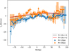 |
Fig. 9. Median Galactocentric vertical velocities (see Paper I, Fig. 15) as a function of the Galactocentric azimuth ϕ (ϕ = 0 marks the direction of the Sun). Solid line stands for the predictions of the warp model at R = 16 kpc described in the text with α = 1 or 2. |
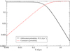 |
Fig. 10. Log-log distribution of probability of the period for the motion of γ(t) = γmax * sin(ωt) and |
8. The Galactic flare
It is well established that stellar kinematics is a fundamental tool to study the dynamics of disks (van der Kruit & Freeman 2011). In this section, we use the basic assumptions behind the Jeans equation, which is that the disk is stationary and axisymmetric. Although, as we discuss below, there is evidence that both these assumptions do not strictly hold and they can be seen as useful working hypotheses. Through the use of the Jeans equation, the dispersion of the vertical velocity, σz, can be related to the thickness of the disk.
8.1. First method
Following van der Kruit (2010), the vertical velocity dispersion for self-gravitating disks can be modeled as
![Mathematical equation: $$ \begin{aligned} \sigma _{\rm z}(R,z) =K\left[ h_{\rm z} \left( 2 - \exp \left(-\mid z \mid / h_{\rm z}\right)\right) \right]^{1/2} \exp \left(- (R - R_\odot )/(2h_{\rm r}) \right) .\end{aligned} $$](/articles/aa/full_html/2020/02/aa36711-19/aa36711-19-eq14.gif) (8)
(8)
López-Corredoira et al. (2002a) give a parametrization for a flared nonwarped Galaxy disk that uses three scale lengths: hr as the horizontal scale length of the stellar distribution in the disk; hz as the vertical scale of the disk that varies with R in an exponential way with a scale hrf as hz = hz0exp((R − R⊙)/hrf). See López-Corredoira et al. (2002a) for details. This parametrization can be combined with Eq. (8) to derive a simple model for the vertical velocity dispersion due to the flaring of the disk alone. By grouping the radial scale lengths, hz and hrf, in a single parameter, H = hrfhr/(hr − hrf), we end up with the equation for the velocity dispersion, σz, to be fit to the data as follows:
![Mathematical equation: $$ \begin{aligned} \begin{array} {l} \sigma _{\rm z} = K \left[ \left( 2 - \exp \left(-\mid z \mid / h_{\rm z}\right)\right) \right]^{1/2} \exp \left((R - R_\odot ) / (2H) \right) \end{array} .\end{aligned} $$](/articles/aa/full_html/2020/02/aa36711-19/aa36711-19-eq15.gif) (9)
(9)
However, the fit using Eq. (9) produces rather poor results and we have explored several alternatives. These bad results have to be expected as Eq. (8) was derived for a pure exponential disk, without flaring that departs from exponential in off-plane regions. As noted by van der Kruit (1988), a pure exponential predicts too large a gradient in velocity dispersion. A modification of Eq. (9) is then proposed as,
 (10)
(10)
We note that K and K′ in Eqs. (9) and (10) account for terms that do not depend on the fitted variables. The expansion series of (2 − exp(−x))1/2 and exp(x/2) coincides with their first two terms for small values of the exponential and differs by x2/2 − x3/4 considering the expansion to fourth order, so the modified function in Eq. (10) reproduces the behavior of Eq. (9) in the plane, while it departs rather markedly off the plane, which is needed to reproduce the observed data.
This model in Eq. 10 was then fit to the data in the anticenter region of Paper I, Fig. 9 bottom panels, from X = 8.4 kpc onwards. Data were averaged in bins of 0.5 kpc in Z and 0.2 kpc in X. The model in Eq. (10) is rather simple and cannot account for the full variability of the observed data. Thus, to avoid oscillations in the model and maintain the physical meaning of the magnitudes, the fitted parameters (hz0, hrf and H) were restricted to a maximum value of 100% above of the corresponding values obtained in López-Corredoira et al. (2002a), while K′ was left free.
The best fit is for χ2 = 12768.4367 with 328 data points. The values for the fitted parameters are: hz0 = 0.3 ± 0.02 kpc; hrf = 5.72 ± 0.34 kpc; and H = 3.05 ± 0.13 kpc, from which a value of hr = 4.90 kpc was derived.
As can be seen in Fig. 11, the agreement is not perfect in any case, and it is better for z > 0 than for z < 0, but in all cases, the trend of the dispersion velocity in the flare model is the same as in the data. Hence a fraction of the observed velocity dispersion can be attributed to the flaring of the disk.
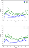 |
Fig. 11. Vertical velocity dispersion for different values of Z (taken from Paper I, Fig. 9) with respect to the X Galactic coordinate. Data from Paper I with their error bars, are represented by crosses; the solid lines are the flare model predictions. Upper panel: for negative Z values, and lower panel: for positive Z values. Same color means same Z. |
8.2. Fit of hz with Moni-Bidin et al. method
We can make a different use of Jeans equations to find a fitting value for the scaleheight hz. We adopted the approach from Moni Bidin et al. (2012), who use two components of Jeans equations to express surface density from Poisson equation in cylindrical coordinates. After making a few assumptions, they obtained an expression for the surface density:
![Mathematical equation: $$ \begin{aligned} \Sigma (z)=\int _{-z}^{z} \rho \mathrm{d} z=\frac{1}{2\pi G}\left[k_1\cdot \int _{0}^{Z} \sigma _{{ v}_R}^2 \mathrm{d} z+ k_2\cdot \int _{0}^{Z} \sigma _{{ v}_{\phi }}^2 \mathrm{d} z \right. \nonumber \\ \left. + k_3\cdot \overline{{ v}_R{ v}_z}+\frac{\sigma _{{ v}_z}^2}{h_z}-\frac{\partial \sigma _{{ v}_z}^2}{\partial z}\right], \end{aligned} $$](/articles/aa/full_html/2020/02/aa36711-19/aa36711-19-eq17.gif) (11)
(11)
where k1, k2, and k3 are constants defined as
 (12)
(12)
We calculated Σ(z) for every R, choosing an initial value of hz = 0.3 kpc. We then proceeded to find the best value of hz for each R, using an iterative method as follows. We did a least squares fit of the theoretical expression Σ = 2ρ(R, z = 0)⋅hz(R)⋅[1 − e−z/hz(R)] with every value of hz from the interval hz ∈ [0, 2] with step Δhz = 0.01. For each value of R, we chose a new value of hz, which corresponds to the smallest χ2. We used this new value of hz to calculate Σ again and we performed a new fit with theoretical the expression for Σ, which yields a new values of hz with minimal χ2 again. We repeated this procedure, until hz converged. We divided R into bins with a size of 0.5 kpc and find the best value of hz for each bin, which gives a dependence hz(R) that we show in the Fig. 12. We fit hz(R) with the linear function, which gives values hz(R) = [(0.370 ± 0.093)+(0.151 ± 0.044)(R( kpc)−R⊙)] kpc, R⊙ = 8.34 kpc. We only calculated hz up to R = 12.0 kpc, as for higher values the fit was imprecise and gave untrustworthy results. We did not use a weighted fit, as the error of Σ(z) is very large, which leads to an incorrect fit. In deriving Eq. (11), it was assumed that  . But, since we are interested in the effect of the flare, we needed to include terms that have not been included so far. This includes dependence hz(R) to Jeans equations and we recalculated the expression for Σ. Then Eq. (11) changes as follows:
![Mathematical equation: $$ \begin{aligned} \Sigma (z)=&\frac{1}{2\pi G}\left[k_1\cdot \int _{0}^{Z} \sigma _{{ v}_R}^2 \mathrm{d} z+ k_2\cdot \int _{0}^{Z} \sigma _{{ v}_{\phi }}^2 \mathrm{d} z + k_3\cdot \overline{{ v}_Rv_z}\right. \nonumber \\&\left. +\frac{\sigma _{{ v}_z}^2}{h_z}-\frac{\partial \sigma _{{ v}_z}^2}{\partial z} +|z| \overline{{ v}_Rv_z}\frac{\partial }{\partial R}\left(\frac{1}{h_z}\right) +\int _{0}^{Z}|z|\frac{\sigma _{R}^2}{R}\frac{\partial }{\partial R}\left(\frac{1}{h_z}\right)\right.\nonumber \\&\left.+\int _{0}^{Z}|z| \sigma _{R}^2\frac{\partial ^2}{\partial R^2}\left(\frac{1}{h_z}\right)\right] .\end{aligned} $$](/articles/aa/full_html/2020/02/aa36711-19/aa36711-19-eq20.gif) (13)
(13)
We repeated the iterative method for new values of Σ and find a new dependence of hz(R). To determine the derivatives of 1/hz in Eq. (13), we used the first result for hz, hz(R) = [0.370 + 0.151(R( kpc)−R⊙)] kpc, derived it, and plugged it in Eq. (13). The resulting relation for hz(R) is plotted in Fig. 13. We fit the new expression for hz(R) with the linear function hz(R) = [(0.533 ± 0.049)+(0.103 ± 0.023)(R( kpc)−R⊙)] kpc.
We see that the effect of the flare causes an increase in hz at the solar radius and decreases the slope of fit of hz(R). Moreover, it is clear that the scale height increases with distance, which is in agreement with results of other authors (Momany et al. 2006; Reylé et al. 2009; López-Corredoira & Molgó 2014; Wang et al. 2018b,c). The effect of the flare is most dominant at high Galactocentric distances (R > 15 kpc), where our method unfortunately gives imprecise results, so we cannot compare these findings. We must bear in mind, however, that this kinematic method gives us information about the mass density (including dark matter) in all components, and not only the stellar density in the disk.
9. A violent origin of the Galactic disk
As we have discussed in the previous sections, the extended analysis of the Gaia mission data has shown that the velocity field of the Milky Way presents large scale gradients in all velocity components. In particular, the radial velocity shows an azimuthal gradient on the order of 40 km s−1 in the galactic plane, ranging from ∼ − 20 km s−1 for 10 kpc ≤ X ≤ 20 kpc and 0 kpc ≤ Y ≤ 20 kpc to ∼20 km s−1 for 10 kpc ≤ X ≤ 20 kpc and −20 kpc ≤ Y ≤ 0 kpc (where X, Y are the galactic coordinates) (Paper I). The tangential velocity also shows a gradient of 40 km s−1 from the orthogonal to parallel direction toward the anticenter. Finally the vertical velocity shows an azimuthal gradient on the order of ∼20 km s−1. The presence of such streaming motions with conspicuous velocity gradients implies that the Milky Way is far from a simple stationary configuration in rotational equilibrium and that axisymmetry is broken.
The dynamical origin of such morphological and velocity features represents an open question that has been investigated by several authors (Antoja et al. 2018; Binney & Schönrich 2018). For instance, Antoja et al. (2018), by studying several phase-space structures in the solar neighborhood, conclude that the Galactic disk is dynamically young so that modeling it as time-independent and axisymmetric is incorrect. In addition they have proposed that the disk must have been tidally perturbed between 300 Myr and 900 Myr ago, which is consistent with estimates of the previous pericentric passage of the Sagittarius dwarf galaxy. In other words, the Galactic disks show features that have been generated less than 1 Gyr ago.
Here, we consider a different perspective about the origin of such nonstationary features; instead of the effect of tidal interactions with neighborhood satellites, we consider a model in which the galactic disk is isolated and has had a relatively violent origin from the monolithic collapse of a protogalactic cloud. Although a model of such a mechanism has not been yet developed in detail for the case of a realistic galactic system, the qualitative results of such collisionless and monolithic gravitational collapses, with and without gas dissipational gas dynamics, are interesting because one can single out some unambiguous signatures of their realizations, as we are going to argue in what follows.
In typical cosmological scenarios (e.g., cold dark-matter-type scenarios), structure formation proceeds hierarchically from very small scales so that self-gravitating particles form quasi-spherical structures, called halos, which have a small angular momentum and a close to isotropic velocity dispersion. The key element in the formation of a disk galaxy is the dissipation associated with nongravitational processes. In particular, gas can dissipate energy through radiative cooling. The effect of such an energy decrease is that it induces the gas to collapse preferentially along its rotational axis, so that it becomes progressively flatter and thus forms a disk. On the other hand, self gravitating particles form through a bottom-up hierarchical aggregation process involving a quasi-spherical configuration with a quasi-isotropic velocity dispersion, that is, the so-called halo structures (Navarro et al. 1997). For this reason, dissipational effects became a necessary ingredient for the formation of disk-like systems. In these kinds of scenarios of disk galaxy formation, there are not rapid and large changes in the system’s physical parameters (mass, size, gravitational potential, etc.). The velocity field of both the gas and the self-gravitating particles, although dominated by rotational and isotropic velocity, respectively, is quiet, that is, there are not large gradients and streaming motions. In particular, the radial velocity is close to zero and the different components of the systems, that is, the halo and the disk, have reached a steady configuration (López-Corredoira et al. 2019). In this situation only an external field, as the one induced by tidal interactions, may generate large scale streaming motions.
When galaxy formation occurs via a top-down monolithic collapse of an isolated over-density, the dynamical evolution is characterized by a phase of rapid and relevant changes of the system’s physical parameters. Given the different dynamical history, the main kinematical features of the states formed are different from those that arise in the hierarchical scenario.
It is well known, since the pioneering work of Lynden-Bell (1967), that an isolated self gravitating overdensity in a nonstationary configuration that rapidly changes its macroscopic properties under the effect of the variation of its own mean field potential until eventually reaching a configuration that is close to a steady state. However, the time scale for a complete relaxation from a generic out-of-equilibrium configuration to a quasi stationary state is poorly constrained both from a theoretical and a numerical point of view.
To explore such a dynamical mechanism, Benhaiem et al. (2017, 2019) studied the properties of the systems formed from the pure gravitational evolution of relatively simple initial conditions (IC). Such systems, although extremely simplified, can give interesting insights as to the dynamics of the monolithic collapse. In this way, it has been shown that when the initial conditions break spherical symmetry and have a nonzero angular momentum, new and almost stationary states appear in which part of the mass continues to evolve for time scales longer than the characteristic collapse time scale  (where ρ is the system’s average mass density). In particular, long-lived non-stationary transients formed with a rich variety of morphological structures, such as spiral arms, bars, shells and even rings that are qualitatively similar to those observed in spiral galaxies. A main feature of such structures is that they are dominated by radial motions that prevent the (fast) relaxation to an equilibrium configuration.
When the IC break spherical symmetry, the gravitational collapse is anisotropic and proceeds faster in the direction of the initial minor semiaxis1. On the other hand, particles that are initially placed along the major semiaxis take longer to arrive at the center and thus they move for a certain time interval in a rapidly varying gravitational field generated by the largest fraction of the mass, which is already re-expanding. In this way, such particles gain kinetic energy in the form of a radial motion so that, although the total energy is conserved, the particle energy distribution largely changes.
Qualitatively the velocity field that results from these simple systems is heterogeneous in nature and strongly scale dependent. In general, there are three regions with different kinematic properties: at small distances from the system center, particles form an extended flattened region that rotates coherently, which is characterized by a relatively large velocity dispersion and for this reason the disk in rather thick. On the other hand, the outermost regions are not axisymmetric and have a radial velocity field directed outwards, which is strongly correlated with the major axis of the system; their energy is still negative but it is close to zero and thus their relaxation time is very long. The extended flattened region dominated by circular motion arises because the collapse is more efficient along the direction parallel to the angular momentum: it is along this direction that the system contracts more.
When gas dynamics is added in the monolithic collapse of an isolated overdensity, different behavior in the inner disk appears. Indeed, the gas is subjected to compression shock and radiative cooling with consequent kinetic and thermal energy dissipation so that it develops a much flatter disk, where rotational motions are coherent and the velocity dispersion is smaller than that of purely self-gravitating particles. In addition, around such a gaseous disk long-lived, but nonstationary, spiral arms formed. On larger scales, where the radial velocity component is significantly larger than the rotational one, the gas follows the same out-of-equilibrium spiral arms traced by purely self-gravitating particles (Sylos Labini et al., in prep.). Thus, even in this case, the violent dynamics characterizing the monolithic collapse of an isolated overdensity naturally give rise to a rather heterogeneous velocity field in which motions are not maximally rotational but characterized by large scales streams in the three velocity components with a predominance of radial motions in the outermost regions of the systems.
Systems formed from the monolithic collapse of an isolated over-density both with and without gas dynamics, show velocity gradients that are generated during the collapse itself, and evolve in time in a nontrivial way. As mentioned above, as the IC break spherical symmetry, the collapse time is different in different directions. In this way, the mechanism of energy gain is also dependent of the direction. For this reason, the system resulting from such a collapse not only shows the heterogeneous velocity field outlined above, but it is characterized by large scale streaming motions. A detailed analysis of this class of systems will be presented in a forthcoming work (Sylos Labini et al., in prep.) but we show in Fig. 14 two examples. The IC consists in a perfect oblate ellipsoid (Run 1) and in an overdensity with an irregular shape (Run 2), respectively. The mass of the systems is M = 1.3 × 10¹⁰ M⊙, their initial gravitational radius is Rg ≈ 10 kpc, and they have the same amount of angular momentum. In this way, their collapse time is τ ≈ 0.1 Gyr. It is important to note that, while this value of the collapse time is fixed by the choice of M and Rg, and thus may be tuned by changing these parameters, the order of the magnitude of the velocity components depend on different properties of the overdensities, most notably on their shape.
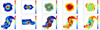 |
Fig. 14. Upper five panels: Run 1, bottom five panels: Runs 2 (see text for details). From left to right: first panel: projection on the X − Y plane (the color code corresponds to the log of the density). Second panel: projection on the X − Z plane (the color code corresponds to the log of the density). Third panel: vertical velocity on the X − Y plane (the color code corresponds to the velocities in km s−1); fourth panel: azimuthal velocity on the X − Y plane (the color code corresponds to the velocities in km s−1). Fifth panel: radial velocity on the X − Y plane (the color code corresponds to the velocities in km s−1). Distances are in kpc. The time is t = 0.6 Gyr. |
Figure 14 shows the two runs at t = 0.6 Gyr (i.e., ≈6 τ): the projection on the X − Y plane (the systems rotates around Z) shows the dense central region (where motion is close to isotropic) surrounded by a less dense flat region where the motion is dominated by the tangential velocity and finally a more sparer outermost region where the radial velocity is dominant. In both cases, there are large scale gradients in the tangential and in the radial velocity but clearly in the case of Run 2, because the IC was less axisymmetric, they have larger amplitude. In particular the radial velocity presents a change from negative to positive, which is an imprint of the collapsing phase where some particles have gained kinetic energy and thus positive radial velocities, and other particles still have radial velocities oriented toward the center and are thus negative. In addition, the vertical velocity also shows large scale gradients, although of smaller amplitude. The time scale of surviving the transient structures depends on the amplitude of the velocity gradients. For instance, a radial velocity gradient of ΔvR ∼ 40 km s−1 implies a change in the disk structure on a time scale on the order of 1 Gyr, given that ΔvR is on the order of 40 kpc Gyr−1 and the disk radius is ∼40 kpc; larger velocity gradients imply a faster evolution.
10. Discussion and conclusions
We explore a variety of dynamical factors that can be tested through the comparison with the extended kinematic maps of Gaia-DR2. Radial and vertical velocities are analyzed here; the analysis of the azimuthal velocities and the derivation of the rotation speed will be treated in a different paper (Paper III).
Many mechanisms may generate either non-null radial velocities or non-null vertical velocities, or there may even be a common origin of some vertical and radial waves (Friske & Schönrich 2019). The gravitational influence of components of the Galaxy that are different from the disk, such as the long bar or bulge, spiral arms, or tidal interaction with Saggitarius dwarf galaxy, may explain some features of the velocity maps, especially in the inner parts of the disk. However, they are not sufficient in explaining the most conspicuous gradients in the outer disk. Vertical motions might be dominated by external perturbations or mergers, although with a minor component due to the warp, as also concluded in the analysis by Wang et al. (2019, 2020) with LAMOST and Gaia data. We carried out N-body simulations to investigate the possible contribution of the minor merger to the vertical asymmetrical bulk motions, and we find that the minor merger with nine satellites can explain the positive vertical velocity on both the north and south side of the hemisphere in the range of 8–18 kpc.
There are two contributions of the warp to the vertical motion: one was produced by the inclination of the orbits, another contribution was from the variation of the amplitude of the warp angle γ. Here, we have detected a non-null variation of the relative amplitude of the warp ( ) that is significant at the 2.6σ level, which is the most likely period for the oscillation of the warp around 0.5 Gyr, although much longer periods are not excluded. Transient warps may be related to a variable torque over the disk; for instance, when the torque is produced by the misalignment of the halo and disk and when the realignment is produced in less than 1 Gyr (Jiang & Binney 1999) or in a scenario of accretion of intergalactic matter with variable ratios of accretion (López-Corredoira et al. 2002b).
Kinematics distributions, including information on the dispersion of velocities, can also be related with the width of the disk. Here, we see with two different methods that the mass distribution of the disk is flared, that is, the thickness of the disk increases outwards. The obtained numbers are roughly consistent with previous analysis of the flare based only on the morphology (and references therein López-Corredoira & Molgó 2014), so we can connect both increasing scaleheight and dispersion of velocities outwards as the same phenomenon. Nonetheless, we must also consider that nonequilibrium systems do not strictly follow the Jeans equation that we have applied in previous sections. Haines et al. (2019) show that traditional Jeans modeling should give reliable results in overdense regions of the disk, but important biases in underdense regions call for the development of nonequilibrium methods to estimate the dynamical matter density locally and in the outer disk. Further analyses of this deviation of Jeans equation in nonequilibrium systems for the application of the present Gaia data will be explored in Paper III.
Precisely, the nonequilibrium system is one of the conclusions of our work here. In lack of other possible causes for the main observed features in the kinematical maps, they can only find an explanation in terms of models in which the Galactic disk is still in evolution, either because the disk has not reached equilibrium since its creation or because external forces, such as the Sagittarius dwarf galaxy, might perturb it. Here, we explore a simple class of out-of-equilibrium, rotating, and asymmetrical mass distributions that evolve under their own gravity. Noncircular orbits and with significant vertical velocities in the outer disk are precisely one of the predictions of this model. Orbits in the very outer disk are out of equilibrium so they have not reached circularity yet, precisely as we observe in our data. The large velocity gradients observed in the Gaia-DR2 data are at odds with the simple model in which stars move on steady circular orbits around the center of the Galaxy. The nonequilibrum model that we discuss provides a first and qualitative framework in which such nonstationarity is intrinsic to the dynamical history of the Galaxy rather than being induced by an ad hoc external field due to the passage of a satellite galaxy.
Certainly, further kinematic information at farther distances or along different lines of sight might better constrain the dynamical scenarios of our Galaxy. Future data releases of Gaia will improve our measurements and analyses, especially if we apply the techniques of extension of kinematic maps using the Lucy’s method for the deconvolution of the parallax errors, as was done in Paper I. On the one hand, the Gaia mission DR3 will provide with more accurate measurements of the parallaxes so that we can make a direct test on the Lucy’s method used on the DR2. On the other hand, such data will allow us to explore the outermost part of the disk for R > 20 kpc where larger velocity gradients are expected according to the nonequilibrium models we have discussed in this work. Also in other galaxies, two-dimensional spectroscopy (for instance, or radio data of THINGS (Sylos Labini et al. 2019), or using Multi Unit Spectroscopic Explorer at the Very Large Telescope) may allow us to carry out an analysis of noncircularity in mean orbits. However, for the case of external galaxies, there is an intrinsic degeneracy between radial and rotational motions if axisymmetry is broken and thus only the direct measurements of the 3D velocity field can clarify the nature of these systems.
The simplest numerical experiments consider ellipsoidal IC where the three semiaxis are a ≥ b ≥ c. More complex shapes must be characterized by the three eigenvalues and eigenvectors of the inertia tensor.
Acknowledgments
Thanks are given to S. Comerón for helpful comments, and Rachel Rudy (language editor of A&A) for proofreading of this text. MLC, FG and ZC were supported by the grant PGC-2018-102249-B-100 of the Spanish Ministry of Economy and Competitiveness (MINECO). HFW is supported by the LAMOST Fellow project, National Key Basic Research Program of China via SQ2019YFA040021 and funded by China Postdoctoral Science Foundation via grant 2019M653504 and Yunnan province postdoctoral Directed culture fundation. HFW is also supported by the Cultivation Project for LAMOST Scientific Payoff and Research Achievement of CAMS-CAS. FSL acknowledges the financial support of the project DynSysMath of the Istituto Italiano di Fisica Nucleare (INFN); this work was granted access to the HPC resources of The Institute for Scientific Computing and Simulation financed by Region Ile de France and the project Equip@Meso (Reference No. ANR-10-EQPX-29-01) overseen by the French National Research Agency as part of the Investissements d’Avenir program. RN was supported by the Scientific Grant Agency VEGA No. 1/0911/17. This work has made use of data from the European Space Agency (ESA) mission Gaia (https://www.cosmos.esa.int/gaia), processed by the Gaia Data Processing and Analysis Consortium (DPAC, https://www.cosmos.esa.int/web/gaia/dpac/consortium). Funding for the DPAC has been provided by national institutions, in particular the institutions participating in the Gaia Multilateral Agreement.
References
- Antoja, T., Helmi, A., Romero-Gómez, M., et al. 2018, Nature, 561, 360 [NASA ADS] [CrossRef] [Google Scholar]
- Benhaiem, D., Joyce, M., & Sylos Labini, F. 2017, ApJ, 851, 19 [NASA ADS] [CrossRef] [Google Scholar]
- Benhaiem, D., Sylos Labini, F., & Joyce, M. 2019, Phys. Rev. E, 99, 022125 [NASA ADS] [CrossRef] [Google Scholar]
- Bennett, M., & Bovy, J. 2019, MNRAS, 482, 1417 [NASA ADS] [CrossRef] [Google Scholar]
- Binney, J., Burnett, B., Kordopatis, G., et al. 2014, MNRAS, 439, 1231 [NASA ADS] [CrossRef] [Google Scholar]
- Binney, J., & Schönrich, R. 2018, MNRAS, 481, 1501 [NASA ADS] [CrossRef] [Google Scholar]
- Binney, J., & Tremaine, S. 2008, Galactic Dynamics, 2nd edn. (Princeton: Princeton Univ. Press) [Google Scholar]
- Bosma, A. 1991, in Warped Disks and Inclined Rings around Galaxies, eds. S. Casertano, P. D. Sackett, & F. H. Briggs, 181 [Google Scholar]
- Bovy, J., Nidever, D. L., & Rix, H.-W. 2014, ApJ, 790, 127 [NASA ADS] [CrossRef] [Google Scholar]
- Bovy, J., Bird, J. C., García Pérez, A. E., Majewski, S. R., Nidever, D. L., & Zasowski, G. 2015, ApJ, 800, 83 [NASA ADS] [CrossRef] [Google Scholar]
- Carrillo, I., Minchev, I., Kordopatis, G., et al. 2018, MNRAS, 475, 2679 [NASA ADS] [CrossRef] [Google Scholar]
- Carrillo, I., Minchev, I., Steinmetz, M., et al. 2019, MNRAS, 490, 797 [Google Scholar]
- Castro-Rodríguez, N., López-Corredoira, M., Sánchez-Saavedra, M. L., & Battaner, E. 2002, A&A, 391, 519 [NASA ADS] [CrossRef] [EDP Sciences] [Google Scholar]
- Drimmel, R., Smart, R. L., & Lattanzi, M. G. 2000, A&A, 354, 67 [NASA ADS] [Google Scholar]
- Faure, C., Siebert, A., & Famaey, B. 2014, MNRAS, 440, 2564 [NASA ADS] [CrossRef] [Google Scholar]
- Friske, J., & Schönrich, R. 2019, MNRAS, 490, 5414 [NASA ADS] [CrossRef] [Google Scholar]
- Gaia Collaboration 2018, A&A, 616, A11 [NASA ADS] [CrossRef] [EDP Sciences] [Google Scholar]
- Gómez, F. A., Minchev, I., O’Shea, B. W., Beers, T. C., Bullock, J. S., & Purcell, C. W. 2013, MNRAS, 429, 159 [NASA ADS] [CrossRef] [Google Scholar]
- Haines, T., D’Onghia, E., Famaey, B., Laporte, C., & Hernquist, L. 2019, ApJ, 879, L15 [NASA ADS] [CrossRef] [Google Scholar]
- Halle, A., Di Matteo, P., Haywood, M., & Combes, F. 2018, A&A, 616, A86 [NASA ADS] [CrossRef] [EDP Sciences] [Google Scholar]
- Hernquist, L. 1990, ApJ, 356, 359 [NASA ADS] [CrossRef] [Google Scholar]
- Hou, L. G., & Han, J. L. 2014, A&A, 569, A125 [NASA ADS] [CrossRef] [EDP Sciences] [Google Scholar]
- Huang, Y., Schönrich, R., Liu, X.-W., et al. 2018, ApJ, 864, 129 [NASA ADS] [CrossRef] [Google Scholar]
- Hunt, J. A. S., Hong, J., Bovy, J., Kawata, D., & Grand, R. J. J. 2018, MNRAS, 481, 3794 [NASA ADS] [CrossRef] [Google Scholar]
- Jiang, I.-G., & Binney, J. 1999, MNRAS, 303, L7 [NASA ADS] [CrossRef] [Google Scholar]
- Kačala, I., Nagy, R., & Klačka, J. 2018, Evolution of Milky Way angular momentum: comparison of the Newtonian gravity with DM and non-Newtonian gravity without DM, (IAU GA 2018, Vienna, Austria), poster session [Google Scholar]
- López-Corredoira, M., & González-Fernández, C. 2016, AJ, 151, 165 [NASA ADS] [CrossRef] [Google Scholar]
- López-Corredoira, M., & Molgó, J. 2014, A&A, 567, A106 [NASA ADS] [CrossRef] [EDP Sciences] [Google Scholar]
- López-Corredoira, M., & Sylos Labini, F. 2019, A&A, 621, A48 [NASA ADS] [CrossRef] [EDP Sciences] [Google Scholar]
- López-Corredoira, M., Cabrera-Lavers, A., Garzón, F., & Hammersley, P. L. 2002a, A&A, 394, 883 [NASA ADS] [CrossRef] [EDP Sciences] [Google Scholar]
- López-Corredoira, M., Betancort-Rijo, J., & Beckman, J. E. 2002b, A&A, 386, 169 [NASA ADS] [CrossRef] [EDP Sciences] [Google Scholar]
- López-Corredoira, M., Abedi, H., Garzón, F., & Figueras, F. 2014, A&A, 572, A101 [NASA ADS] [CrossRef] [EDP Sciences] [Google Scholar]
- López-Corredoira, M., Sylos Labini, F., Kalberla, P. M. W., & Allende Prieto, C. 2019, AJ, 157, 26 [NASA ADS] [CrossRef] [Google Scholar]
- Lynden-Bell, D. 1967, MNRAS, 167, 101 [NASA ADS] [CrossRef] [Google Scholar]
- Macciò, A. V., Dutton, A. A., & van den Bosch, F. C. 2008, MNRAS, 391, 1940 [NASA ADS] [CrossRef] [Google Scholar]
- McGaugh, S. S., Lelli, F., & Schombert, J. M. 2016, Phys. Rew. Lett., 117, 201101 [CrossRef] [Google Scholar]
- Miyamoto, M., & Zhu, Z. 1998, AJ, 115, 1483 [NASA ADS] [CrossRef] [Google Scholar]
- Miyamoto, M., Soma, M., & Yoshizawa, M. 1993, AJ, 105, 2138 [NASA ADS] [CrossRef] [Google Scholar]
- Momany, Y., Zaggia, S., Gilmore, G., Piotto, G., Carraro, G., Bedin, L. R., & De Angeli, F. 2006, A&A, 451, 515 [NASA ADS] [CrossRef] [EDP Sciences] [Google Scholar]
- Monari, G., Helmi, A., Antoja, T., & Steinmetz, M. 2014, A&A, 569, A69 [NASA ADS] [CrossRef] [EDP Sciences] [Google Scholar]
- Monari, G., Famaey, B., & Siebert, A. 2016, MNRAS, 457, 2569 [NASA ADS] [CrossRef] [Google Scholar]
- Moni Bidin, C., Carraro, G., Méndez, R. A., & Smith, R. 2012, ApJ, 751, 30 [NASA ADS] [CrossRef] [Google Scholar]
- Moster, B. P., Naab, T., & White, S. D. M. 2013, MNRAS, 428, 3121 [NASA ADS] [CrossRef] [Google Scholar]
- Navarro, J. F., Frenk, C. S., & White, S. D. M. 1997, ApJ, 490, 493 [NASA ADS] [CrossRef] [Google Scholar]
- Poggio, E., Drimmel, R., Lattanzi, M. G., et al. 2018, MNRAS, 481, L21 [NASA ADS] [CrossRef] [Google Scholar]
- Quillen, A. C., Carrillo, I., Anders, F., et al. 2018, MNRAS, 480, 3132 [NASA ADS] [CrossRef] [Google Scholar]
- Reylé, C., Marschall, D. J., Robin, A. C., & Schultheis, M. 2009, A&A, 495, 819 [NASA ADS] [CrossRef] [EDP Sciences] [Google Scholar]
- Romero-Gómez, M., Mateu, C., Aguilar, L., Figueras, F., & Castro-Ginard, A. 2019, A&A, 627, A150 [NASA ADS] [CrossRef] [EDP Sciences] [Google Scholar]
- Ruchti, G. R., Read, J. I., Feltzing, S., Pipino, A., & Bensby, T. 2014, MNRAS, 444, 515 [Google Scholar]
- Ruchti, G. R., Read, J. I., Feltzing, S., et al. 2015, MNRAS, 450, 2874 [NASA ADS] [CrossRef] [Google Scholar]
- Siebert, A., Famaey, B., & Minchev, I. 2011, MNRAS, 412, 2026 [NASA ADS] [CrossRef] [Google Scholar]
- Sylos Labini, F., Benhaiem, D., Comerón, S., & López-Corredoira, M. 2019, A&A, 622, A58 [NASA ADS] [CrossRef] [EDP Sciences] [Google Scholar]
- Tian, H.-J., Liu, C., Wan, J.-C., et al. 2017, RAA, 17, 114 [NASA ADS] [Google Scholar]
- Vallée, J. P. 2017, Astron. Rev., 13, 113 [Google Scholar]
- van der Kruit, P. C. 1988, A&A, 192, 117 [NASA ADS] [Google Scholar]
- van der Kruit, P. C. 2010, in American Institute of Physics Conference Series, eds. V. P. Debattista, & C. C. Popescu, Am. Inst. Phys. Conf. Ser., 1240, 387 [NASA ADS] [Google Scholar]
- van der Kruit, P. C., & Freeman, K. C. 2011, ARA&A, 49, 301 [NASA ADS] [CrossRef] [Google Scholar]
- Wang, H. F., Carlin, J. L., Huang, Y., et al. 2019, ApJ, 884, 135 [NASA ADS] [CrossRef] [Google Scholar]
- Wang, H. F., Liu, C., Deng, L. C., et al. 2018c, in Rediscovering our Galaxy, eds. C. Chiappini, I. Minchev, E. Starkenberg, M. Valentini, et al. (Cambridge: Cambridge Univ. Press), IAU Symp., 334, 378 [NASA ADS] [Google Scholar]
- Wang, H. F., López-Corredoira, M., Carlin, J. L., et al. 2018a, MNRAS, 477, 2858 [NASA ADS] [CrossRef] [Google Scholar]
- Wang, H. F., Liu, C., Xu, Y., et al. 2018b, MNRAS, 478, 3367 [NASA ADS] [CrossRef] [Google Scholar]
- Wang, H. F., López-Corredoira, M., Huang, Y., et al. 2020, MNRAS, 491, 2104 [NASA ADS] [Google Scholar]
- Wang, L., Dutton, A. A., Stinson, G. S., et al. 2015, MNRAS, 454, 83 [NASA ADS] [CrossRef] [Google Scholar]
- Weinberg, M. D. 1991, ApJ, 373, 391 [NASA ADS] [CrossRef] [Google Scholar]
- Widrow, L. M., Gardner, S., Yanny, B., Dodelson, S., & Chen, H.-Y. 2012, ApJ, 750, L41 [NASA ADS] [CrossRef] [Google Scholar]
- Yuan, Z., Chang, J., Banerjee, P., et al. 2018, ApJ, 863, 26 [NASA ADS] [CrossRef] [Google Scholar]
All Figures
|
Fig. 1. Left: Gaia extended kinematic maps (Fig. 8 of Paper I) with the over-plotting of the representation of the spiral arms: four main spiral arms follow the model of Vallée (2017) and the local spur modeled by Hou & Han (2014): upper panel, radial velocity; bottom panel, vertical velocity. Right: Gaia extended kinematic maps introducing a correction to the zero-point bias of parallaxes πc = π + 0.03 mas (Fig. 16 of Paper I). |
| In the text | |
|
Fig. 2. Bending and breathing velocities, using the same graphic layout and panel distribution as in GC18. Left column panels: bending vertical velocity; middle column panels: breathing vertical velocities; and right column panels: error in the computed values for both bending and breathing modes. Units of velocities in km s−1; units of scale X, Y in kpc. Position of the Sun at X = 8.34, Y = 0; position of the Galactic center at X = 0, Y = 0. See text. |
| In the text | |
|
Fig. 3. Mean value of radial velocity over various z intervals as a function of the Galactocentric distance along the center-Sun-anticenter direction using data by Paper I. |
| In the text | |
|
Fig. 4. Mean value of radial velocity as a function of Y for various values of X by using data from Paper I. |
| In the text | |
|
Fig. 5. Mean value of radial velocity as a function of Y for various values of X by using results of integration of 105 test particles in the rotating gravitational potential of the Galactic bar considering Newtonian dynamics. |
| In the text | |
|
Fig. 6. Mean value of radial velocity as a function of Y for various values of X by using results of integration of 105 test particles in the rotating gravitational potential of the Galactic bar considering MOND. |
| In the text | |
|
Fig. 7. Edge−on views of the kinematics of the disk with range of 8.5−17.5 kpc, shown as median velocity maps of VZ (in km−1) in the N-body simulation. There are clear vertical bulk motions or bending mode motions in the range of 10−17 kpc; especially for Z when less than 2 kpc. |
| In the text | |
|
Fig. 8. Edge−on views of the kinematics of the disk with range of R = 8–20 kpc and Z = −2.5–2.5 kpc, shown as median velocity maps of VZ (in km−1) for different azimuthal angles in the N-body simulation. Colors and labels are the same as in Fig. 7. |
| In the text | |
|
Fig. 9. Median Galactocentric vertical velocities (see Paper I, Fig. 15) as a function of the Galactocentric azimuth ϕ (ϕ = 0 marks the direction of the Sun). Solid line stands for the predictions of the warp model at R = 16 kpc described in the text with α = 1 or 2. |
| In the text | |
|
Fig. 10. Log-log distribution of probability of the period for the motion of γ(t) = γmax * sin(ωt) and |
| In the text | |
|
Fig. 11. Vertical velocity dispersion for different values of Z (taken from Paper I, Fig. 9) with respect to the X Galactic coordinate. Data from Paper I with their error bars, are represented by crosses; the solid lines are the flare model predictions. Upper panel: for negative Z values, and lower panel: for positive Z values. Same color means same Z. |
| In the text | |
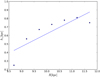 |
Fig. 12. Fit of hz as a function of Galactocentric radius derived with Eq. (11). |
| In the text | |
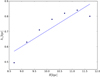 |
Fig. 13. Same as Fig. 12, but after correction with flare as given in Eq. (13). |
| In the text | |
|
Fig. 14. Upper five panels: Run 1, bottom five panels: Runs 2 (see text for details). From left to right: first panel: projection on the X − Y plane (the color code corresponds to the log of the density). Second panel: projection on the X − Z plane (the color code corresponds to the log of the density). Third panel: vertical velocity on the X − Y plane (the color code corresponds to the velocities in km s−1); fourth panel: azimuthal velocity on the X − Y plane (the color code corresponds to the velocities in km s−1). Fifth panel: radial velocity on the X − Y plane (the color code corresponds to the velocities in km s−1). Distances are in kpc. The time is t = 0.6 Gyr. |
| In the text | |
Current usage metrics show cumulative count of Article Views (full-text article views including HTML views, PDF and ePub downloads, according to the available data) and Abstracts Views on Vision4Press platform.
Data correspond to usage on the plateform after 2015. The current usage metrics is available 48-96 hours after online publication and is updated daily on week days.
Initial download of the metrics may take a while.