| Issue |
A&A
Volume 627, July 2019
|
|
|---|---|---|
| Article Number | A76 | |
| Number of page(s) | 8 | |
| Section | The Sun | |
| DOI | https://doi.org/10.1051/0004-6361/201935515 | |
| Published online | 03 July 2019 | |
Quasilinear approach of the cumulative whistler instability in fast solar wind: Constraints of electron temperature anisotropy
1
Centre for Mathematical Plasma Astrophysics, Celestijnenlaan 200B, 3001 Leuven, Belgium
e-mail: shaaban.mohammed@kuleuven.be
2
Theoretical Physics Research Group, Physics Department, Faculty of Science, Mansoura University, Mansoura 35516, Egypt
3
Institut für Theoretische Physik, Lehrstuhl IV: Weltraum- und Astrophysik, Ruhr-Universität Bochum, 44780 Bochum, Germany
4
Institute for Physical Science and Technology, University of Maryland, College Park, MD 20742, USA
5
Korea Astronomy and Space Science Institute, Daejeon 34055, Korea
6
School of Space Research, Kyung Hee University, Yongin, Gyeonggi 17104, Korea
Received:
21
March
2019
Accepted:
25
May
2019
Context. Solar outflows are a considerable source of free energy that accumulates in multiple forms such as beaming (or drifting) components, or temperature anisotropies, or both. However, kinetic anisotropies of plasma particles do not grow indefinitely and particle-particle collisions are not efficient enough to explain the observed limits of these anisotropies. Instead, self-generated wave instabilities can efficiently act to constrain kinetic anisotropies, but the existing approaches are simplified and do not provide satisfactory explanations. Thus, small deviations from isotropy shown by the electron temperature (T) in fast solar winds are not explained yet.
Aims. This paper provides an advanced quasilinear description of the whistler instability driven by the anisotropic electrons in conditions typical for the fast solar winds. The enhanced whistler-like fluctuations may constrain the upper limits of temperature anisotropy A ≡ T⊥/T∥ > 1, where ⊥, ∥ are defined with respect to the magnetic field direction.
Methods. We studied self-generated whistler instabilities, cumulatively driven by the temperature anisotropy and the relative (counter)drift of electron populations, for example, core and halo electrons. Recent studies have shown that quasi-stable states are not bounded by linear instability thresholds but an extended quasilinear approach is necessary to describe these quasi-stable states in this case.
Results. Marginal conditions of stability are obtained from a quasilinear theory of cumulative whistler instability and approach the quasi-stable states of electron populations reported by the observations. The instability saturation is determined by the relaxation of both the temperature anisotropy and relative drift of electron populations.
Key words: instabilities / plasmas / solar wind / Sun: coronal mass ejections / Sun: flares
© ESO 2019
1. Introduction
Solar wind expansion is governed by mechanisms that trigger the escape of coronal plasma particles and those that self-regulate more violent outflows such as coronal mass ejections or fast winds. One of the still intriguing questions contrasting the main features of fast and slow winds is electron temperature anisotropy. Deviations from isotropy shown by the electron temperature in the fast wind (VSW > 500 km s−1) are much lower than those measured in the slow winds (Štverák et al. 2008), suggesting the existence of an additional constraining factor. In the slow winds (VSW < 500 km s−1) the relative drift between thermal (core) and suprathermal (halo) electrons is negligibly small and it was relatively straightforward to show that large deviations from isotropy are mainly constrained by self-generated temperature-anisotropy instabilities (Štverák et al. 2008; Lazar et al. 2017a; Shaaban et al. 2019a). In this case whistler modes are destabilized by a temperature anisotropy A ≡ T⊥/T∥ > 1, where ⊥ and ∥ denote directions with respect to the local magnetic field. The situation is however different in fast winds, where the core-halo drift increases mainly owing to an enhancement of electron strahl or heat-flux population. These (counter-)drifting components can be at the origin of so-called heat-flux instabilities (Gary 1985; Saeed et al. 2017; Shaaban et al. 2018a,b; Tong et al. 2019), which usually are considered responsible for strahl isotropization and loss of intensity with solar wind expansion and increasing distance from the Sun (Maksimovic et al. 2005; Vocks et al. 2005; Pagel et al. 2007). If the self-generated instabilities play a role in the limitation of temperature anisotropy in this case, electron strahl and heat-flux instabilities must contribute as well.
Heat-flux instabilities can manifest either as a whistler unstable mode, when the relative drift is small, or as a firehose instability driven by more energetic beams with a relative drift exceeding thermal velocity of beaming electrons (Gary 1985; Shaaban et al. 2018a,b). Solar wind conditions are in general propitious to whistler heat-flux instability (WHFI; Viñas et al. 2010; Bale et al. 2013; Shaaban et al. 2018a; Tong et al. 2019), and recent studies have unveiled various regimes triggered by the interplay with temperature anisotropy of electrons (Shaaban et al. 2018b). Thus, the unstable whistlers are inhibited by increasing the relative drift (or beaming) velocity, but are stimulated by a temperature anisotropy A ≡ T⊥/T∥ > 1 (Shaaban et al. 2018b). In this paper we investigate the whistler anisotropy-driven instability for contrasting conditions in slow and fast solar winds. As already mentioned, in slow winds the relative drifts between electron populations are small and predictions made for non-drifting components are found satisfactory (Štverák et al. 2008; Lazar et al. 2017a; Shaaban et al. 2019a). On the other hand, in fast winds two sources of free energy may coexist and interplay, and in this case the instability is cumulatively driven by temperature anisotropy under the influence of the relative core-halo drift. In turn, the enhanced fluctuations are expected to act and constrain the temperature anisotropy and eventually explain boundaries reported by observations in fast winds.
However, if the instability results from the interplay of two sources of free energy threshold, conditions provided by a linear approach may have a reduced relevance. Such a critical feature is suggested by recent quasilinear (QL) studies of the WHFI driven by the relative drift of the core and halo electrons (Shaaban et al. 2019b). These studies show instability saturation emerging from a concurrent effect of the induced anisotropies, i.e., Ac > 1 for the core and Ah < 1 for the beam (or halo), through heating and cooling processes, and an additional minor relaxation of drift velocities. It then becomes clear that linear theory cannot describe such an energy transfer between electron populations and cannot characterize the quasi-stable states reached after relaxation (Shaaban et al. 2018a, 2019b). We present the results of an extended QL analysis of the cumulative whistler instability (WI), providing valuable insights about the instability saturation via a complex relaxation of the relative drift between core and halo electrons and their temperature anisotropy.
The present manuscript is structured as follows: The electron velocity distribution function (eVDF) is introduced in Sect. 2 inspired by observations in slow and fast solar winds, which show two counter-drifting anisotropic core and halo electron populations. In Sect. 3 we present in brief the QL approach used to describe a cumulative whistler anisotropy-driven instability in the solar wind conditions. Relevant numerical solutions are discussed in Sect. 4, showing the influence of initial conditions (e.g., temperature anisotropy and (counter-)drifting velocities), on the subsequent evolutions of both the core and halo parameters (e.g., plasma betas, drift velocities, and the associated electromagnetic fluctuations). Finally, the new results from our QL analysis are compared with the observational upper limits of electron temperature anisotropies, for both the core and halo populations and both slow and fast wind conditions. The results of this work are summarized in Sect. 5.
2. Solar wind electrons
In the solar wind the eVDFs are well reproduced by a core-halo model (Maksimovic et al. 2005; Štverák et al. 2008; Pierrard et al. 2016; Lazar et al. 2017b; Tong et al. 2019)

where δ = nh/n0, 1 − δ = nc/n0 are the halo and core relative densities, respectively, and n0 ≡ ne is the total number density of electrons. A relative core-halo drift becomes more apparent during the fast winds (VSW > 500 km s−1), such that, with respect to their center of mass the core can be described by a drifting bi-Maxwellian, while the halo by another counter-drifting bi-Maxwellian or bi-kappa distribution (Maksimovic et al. 2005; Štverák et al. 2008). In order to keep the analysis transparent (away from suprathermal effects) we assume both the core (subscript a = c) and halo (a = h) populations well described by drifting bi-Maxwellians (Saeed et al. 2017; Tong et al. 2018; Shaaban et al. 2018b), i.e.,
with a drifting velocity Ua (along the background magnetic field) in the frame of the mass center, for example, fixed to protons (a = p), which are assumed non-drifiting Maxwellian (Up = 0); the expression α∥, ⊥, a(t) is related to the components of (kinetic) temperature (which may vary in time, t), i.e.,
The net current is preserved zero by restricting to ncUc + nhUh = 0 in a quasi-neutral electron-proton plasma with ne ≈ np. In the slow wind conditions (VSW < 500 km s−1) the relative drifts are small and can be neglected, i.e., Ua = 0.
In the present analysis plasma parameterization is based on observational data provided in recent decades by various missions, for example, Ulysses, Helios 1, Cluster II, and Wind (Maksimovic et al. 2005; Štverák et al. 2008; Pulupa et al. 2014; Pierrard et al. 2016; Tong et al. 2018). In slow wind conditions (VSW < 500 km s−1), Ua ≃ 0 and the observed quasi-stable states and their temperature anisotropy A = T⊥/T∥ > 1 are well constrained by the self-generated non-drifting WI (Štverák et al. 2008; Lazar et al. 2018a). On the other hand, for the fast wind conditions (VSW > 500 km s−1) the limits of temperature anisotropy A = T⊥/T∥ > 1, for both the core and halo populations, are constrained to lower limits, much below the existing predictions for non-drifting models (Štverák et al. 2008).
In situ measurements also reveal a cooler electron core (Tc < Th), but this core is more dense than halo population and has an average number density nc = 0.95 n0 (Maksimovic et al. 2005; Štverák et al. 2008; Pierrard et al. 2016). Both populations may show comparable temperature anisotropies, i.e., Ac ∼ Ah, which trigger different instabilities such as the WI ignited by T⊥ > T∥ or firehose instabilities driven by T∥ > T⊥ (Pierrard et al. 2016; Lazar et al. 2018a). Recent reports using Wind data have suggested that the core drift velocity is comparable to, or larger than the Alfvén speed  (implying
  at electron scales, where μ = mp/me is the proton–electron mass ratio) (Pulupa et al. 2014; Tong et al. 2018). As mentioned in the Introduction, the core–halo relative drift velocity can be source of beaming instabilities, such as WHFI and firehose-like instabilities (Gary 1985; Saeed et al. 2017; Shaaban et al. 2018a,b; Tong et al. 2019). Values adopted in this work for the relative drift velocities are sufficiently small, for example,
  , to guarantee a whistler unstable regime (with a major stimulating effect of the heat flux; see Shaaban et al. 2018b) and allow us to compare our results with the observations showing the limits of temperature anisotropy A = T⊥/T∥ > 1 reported in Štverák et al. (2008). To be consistent with our model in Eq. (2) we selected only the events associated with thermalized halo components, i.e., described by a κ-distribution with large enough κ > 6. Plasma parameters (dimensionless) adopted as initial conditions in our present analysis are tabulated in Table 1, unless otherwise specified.
Parameters for the halo and core electron populations.
3. Quasilinear theory
In a collisionless and homogeneous electron-proton plasma the linear (instantaneous) dispersion relation describing whistler modes (Shaaban et al. 2018b) is written as
![$$ \begin{aligned} \tilde{k}^2&=(1-\delta )\, \left[\Lambda _{\rm c}+\frac{(\Lambda _{\rm c}+1)\,(\tilde{\omega }-\tilde{k}\,u_{\rm c}) - \Lambda _{\rm c}}{\tilde{k} \sqrt{\beta _{\rm c}}} Z_{\rm c}\left(\frac{\tilde{\omega }-1-\tilde{k}\,u_{\rm c}}{\tilde{k} \sqrt{\beta _{\rm c}}}\right)\right]\nonumber \\&\quad + \delta \,\left[\Lambda _{\rm h}+\frac{(\Lambda _{\rm h}+1)\,(\tilde{\omega }-\tilde{k}\,u_{\rm h}) - \Lambda _{\rm h}}{\tilde{k} \sqrt{\beta _{\rm h}}} Z_h\left(\frac{\tilde{\omega }-1-\tilde{k}\,u_{\rm h}}{\tilde{k} \sqrt{\beta _{\rm h}}}\right)\right]\nonumber \\&\quad +\frac{\tilde{\omega }}{\tilde{k}\,\sqrt{\mu \,\beta _{\rm p}}}Z_{\rm p}\left(\frac{\mu \,\tilde{\omega }+1}{\tilde{k}\sqrt{\mu \,\beta _{\rm p}}}\right), \end{aligned} $$](/articles/aa/full_html/2019/07/aa35515-19/aa35515-19-eq7.gif)
where k̃ = kc/ωp,e is the normalized wave number k, c is the speed of light,  is the plasma frequency of electrons,
  is the normalized wave frequency, Ωe is the nonrelativistic gyro-frequency of electrons, Λa = Aa − 1,
  are the plasma beta parameters for protons (subscript “a = p”), electron core (subscript “a = c”), and electron halo (subscript “a = h”) populations, ua = μ−1/2Ua/vA are normalized drifting velocities,
  is the Alfvén speed, and
is the plasma dispersion function (Fried & Conte 1961).
Beyond the linear theory, we solve QL equations for both particles and electromagnetic waves. For transverse modes propagating parallel to the magnetic field, the particle kinetic equation for electrons in the diffusion approximation is given by (Seough & Yoon 2012; Shaaban et al. 2019b)
![$$ \begin{aligned} \frac{\partial f_a}{\partial t}&=\frac{i e^2}{4m_a^2 c^2}\int _{-\infty }^{\infty } \frac{\mathrm{d}k}{k}\left[ \left(\omega ^*-k { v}_\parallel \right)\frac{\partial }{{ v}_\perp \,\partial { v}_\perp }+ k\frac{\partial }{\partial { v}_\parallel }\right]\nonumber \\&\quad \times \,\frac{ { v}_\perp ^2\,\delta B^2(k, \omega )}{\omega -k{ v}_\parallel -\Omega _a}\left[ \left(\omega -k v_\parallel \right)\frac{\partial }{{ v}_\perp \,\partial { v}_\perp }+ k \frac{\partial }{\partial { v}_\parallel }\right]f_a, \end{aligned} $$](/articles/aa/full_html/2019/07/aa35515-19/aa35515-19-eq13.gif)
where δB2(k) is the energy density of the fluctuations described by the wave kinetic equation
and γk is the instability growth rate calculated from Eq. (4). Dynamical kinetic equations for the velocity moments of the distribution function, such as temperature components T⊥, ∥ a of core (a = c) and halo (a = h) and their drift velocities Ua, are given by
Detailed derivations of Eq. (8) can be found in Seough & Yoon (2012), Yoon et al. (2012), Sarfraz et al. (2016), Lazar et al. (2018b), Shaaban et al. (2019a), Shaaban et al. (2019b).
4. Cumulative whistler instability
In this section we examine the WI cumulatively driven by anisotropic temperature (Aa > 1) and (counter-)drifting motion of the core and halo electrons. For electrons with anisotropic temperature Ae > 1 and no drifting components, both theory and simulations predict the excitation of parallel whistlers that rapidly consumes most of the free energy before the electron mirror instability can grow with a considerable growth rate (Gary & Karimabadi 2006; Ahmadi et al. 2016). In turn, the electron anisotropy is bounded by WI that scatters electrons and imposes a β∥-dependent upper bound on the instability thresholds (Gary & Karimabadi 2006), which shapes the anisotropy limits reported by the observations in the slow wind (Štverák et al. 2008; Adrian et al. 2016). Motivated by these premises, and by the assumption of small drifts, which inhibit mirror modes but may stimulate whistlers (Shaaban et al. 2018b), in the present study we analyzed only the whistler modes propagating parallel to the magnetic field. We note that a WHFI can be excited only for a modest drift velocity that is lower than thermal speed, i.e., uh < vres (Gary 1985; Shaaban et al. 2018a). Both WI and WHFI have the same dispersive characteristics because they are triggered by resonant halo electrons and exhibit maximum growth rates for parallel propagation (Gary & Karimabadi 2006; Shaaban et al. 2018b). Linear properties of these two distinct regimes have recently been contrasted and discussed in detail in Shaaban et al. (2018b), showing that all dispersive features are markedly altered by the interplay of electron anisotropies, namely their temperature anisotropy and drifting velocities. In this section we present the results from an extended QL analysis that is able to characterize the long-run time evolution of the enhanced fluctuations, including their saturation and back reaction on both the core and halo populations.
4.1. Quasilinear results
We resolve the set of QL Eqs. (7) and (8) for the initial parameters (τ = 0) in Table 1. To do so, we use a discrete grid in the positive normalized wave-number k̃-space, i.e., 0.1 < k̃ < 1.6, where Nk = 400 points separated by dk∼ = 0.04. The initial wave spectrum is assumed to be constant over the initially unstable k̃-space (Yoon 1992) and we adopted an arbitrary value of 5 × 10⁻⁶. The linear (instantaneous) dispersion relation (4) for WI can be solved using the plasma parameters and magnetic wave energy at time step τ = t|Ωe|. The results at this moment are the unstable solutions of the WI, i.e., growth rate and wave frequency as functions of k̃. By using these solutions we then compute the integrals defined in the QL equations and evaluate the time derivative of each plasma parameters for both the core and halo populations. Then we allow the whole system to evolve to the next step τ + dτ using the second order leapfrog-like method. Numerical integration is performed between 0 ≤ τ ≤ 1500 with time step of dτ = 0.1. It is well known that such plasma systems conserve momentum and energy; this corresponds to the sum of the plasma particles energies, i.e., temperatures and drifts velocities, and plasma waves energy. Excess of plasma particle free energies drives instabilities, thereby enhancing the electromagnetic fluctuations, i.e., the wave energy. In turn, the enhanced fluctuations scatter particles to the quasi-stable state, reducing the anisotropy of particle distributions through wave-particle interaction (Moya et al. 2011; Yoon et al. 2012; Shaaban et al. 2019b; López et al. 2019). Figure 1 shows temporal profiles for the plasma beta parameters ( ), parallel (red) and perpendicular (blue) components for the halo (subscript h) and core (subscript c) populations, and their drift velocities uh, c, and the corresponding increase of the wave magnetic power
  (bottom). We consider the core initially isotropic (Ac(0) = 1), and halo with Ah(0) = 4.0 and initial drifts defining three cases: uh(0) = 0.0 (left), 0.25 (middle), and 0.5 (right). The effects of whistler fluctuations on the core and halo populations can be explained by the resonant heating and cooling mechanisms, combined with an adiabatic scattering and diffusion of particles in velocity space. Initially anisotropic, the halo electrons are subject to perpendicular cooling (blue) and parallel heating (red), while the isotropic core electrons experience perpendicular heating (blue) and parallel cooling (red). After relaxation, both components end up with small (and similar) temperature anisotropies. Moreover, drift velocities reduce in time to lower but finite values. It is worth outlining the advantage of using a QL analysis that can unveil the energy transfer between electron populations during the instability excitation; for example, the initially isotropic core gains free energy, i.e., temperature anisotropy in perpendicular direction β⊥ c > β∥ c. If the halo drift velocity is initially higher, i.e., uh(0) = 0.5 (right panels), all temporal variations change, namely, the halo becomes less anisotropic, the initially isotropic core (Ac(0) = 1.0) becomes more anisotropic (Ac > 1.0), and the level of saturated fluctuations increases. By comparison to the first case without drifts (uh = 0.0), all these processes (and mechanisms involved) are delayed in time by a factor of ∼1.5 for uh = 0.25 and ∼3 for uh = 0.5. This delay is consistent with predictions from linear theory that show an inhibition of whistlers, where maximum (peaking) growth rates decrease for finite drifts by a factor of ∼1.5 for uh = 0.25 and ∼3 for uh = 0.5; see, for instance, Fig. 3 in Shaaban et al. (2018b).
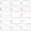 |
Fig. 1. Time evolutions for three distinct initial conditions uh(0) = 0.0 (left column), uh(0) = 0.25 (middle column), and uh(0) = 0.5 (right column), for β⊥ a (solid blue) and, and β∥ a (solid red) for core (a = c) and halo electrons (a = h), and their drift velocities ua, and the wave energy density (solid black). |
Figure 2 presents temporal profiles for the same plasma parameters, but for different initial conditions assuming that both halo and core electrons possess similar initial anisotropies Ah(0) ≃ Ac(0) = 4.0. The rest of the initial plasma parameters are the same as in Fig. 1. In this second case, both the core and halo electrons reduce their temperature anisotropies and drift velocities, leading to higher wave powers at the saturation. An initially anisotropic core (Ac(0) = 4.0) determines a faster relaxation. These results are in perfect agreement with recent studies that strongly suggest that electron kinetic instabilities are markedly stimulated by the interplay of the core and halo temperature anisotropies (Lazar et al. 2018a; Shaaban et al. 2019a). A higher initial drift uh(0) = 0.5 has visible consequences on the temperature anisotropy of halo electrons, which decreases to lower values, but only slightly affects the time evolution of the core anisotropy. Predictions from linear theory show a similar influence of the drift velocity on the WI driven by the temperature anisotropy. Increasing the halo drift velocity uh stimulates the instability driven by the core anisotropy (Ac > 1), but inhibits the fluctuations triggered by the halo anisotropy (Ah > 1) (Shaaban et al. 2018b). For cases with uh ≠ 0, the relaxation of the drift velocity contributes to isotropization of the halo electrons and to an increase of the core anisotropy that feeds the instability and enhances the wave energy. This complex scenario may be explained by a transfer of energy and momentum between core and halo electrons and the enhanced fluctuations.
4.2. Constraints on the observed temperature anisotropies
In order to emphasize the importance of the present study, in this section we perform a comparative analysis of the new anisotropy thresholds predicted by our QL approach for the cumulative WI and temperature anisotropy of quasi-stable states, as reported by the observations of solar wind electrons. The observational data set is selected from roughly 120 000 events detected in the ecliptic by three spacecrafts, Helios I, Cluster II, and Ulysses at different heliocentric distances from the Sun, i.e., 0.3−3.95 AU. Figures 3 and 4 show the observational data for the electron populations from slow (with VSW < 500 km s−1) and fast winds (with VSW > 500 km s−1), respectively. Distinction is also made between halo (left panels) and core (right panels) electron populations. As already mentioned, these observational data are selected from the events associated with thermalized halo components (described by a κ-distribution with large enough κ > 6), for which the effects of the suprathermal populations on the QL saturation of WI and the relaxation of the anisotropic distribution are only minor (Lazar et al. 2018b). Occurrence rates showing the number of events in bins of temperature anisotropies T⊥ a/T∥ a versus parallel plasma beta  (subscript “a = h” for halo and “a = c” for core) are color coded using a blue-green-yellow color scheme. Unlike the results obtained by Adrian et al. (2016), using a bulk model of the solar wind electrons, our calculations are based on a realistic dual model, which captures not only the effects of temperature anisotropy but also the influence of the core–halo relative drift characteristic to fast winds.
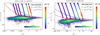 |
Fig. 3. Linear WI thresholds and QL dynamical paths of temperature anisotropy Ah, c derived for uh = 0.0, are compared with the quasi-stable states of electron halo (left) and core (right) populations from slow winds (VSW < 500 km s−1). |
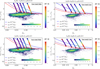 |
Fig. 4. Linear WI thresholds and QL dynamical paths of temperature anisotropy Ah, c derived for uh = 0.25 (top) and 0.5 (bottom) compared with the quasi-stable states of the electron halo (left) and core (right) populations from fast winds (VSW > 500 km s−1). |
The observational data are contrasted with the anisotropy thresholds of WI as resulted from the interplay of the halo and core electron populations for non-drifting velocities uh = 0 in Fig. 3 and finite drifts uh ≠ 0 in Fig. 4. These thresholds are derived for different maximum growth rates γm/|Ωe|=10−2, 10−3, 10−4, and are described with a general fitting law (Lazar et al. 2014)
Fitting parameters a, b, c, and d are tabulated in Tables 2–4.
Figure 3 enables a comparison of observational data, halo (left), and core (right) electron populations from slow winds (VSW < 500 km s−1 and ua = 0) with the WI thresholds and the QL dynamical paths obtained for different initial plasma betas, i.e.,  , and
, and  , in a
  diagram. The initial positions, i.e.,
  , are indicated by blue-filled circles, while after saturation the final positions, i.e.,
  , are indicated by red-filled circles. The levels of the wave energy density
  are coded with a “rainbow” color scheme. We observe that the initial anisotropies are reduced in time toward quasi-stable regimes and end up exactly at the WI threshold with a maximum growth rate γm = 10−3|Ωe| (red line) predicted by the linear theory. To be consistent with our dual model in Eq. (2) the electron data is more selective and more restrictive than the data set used in Štverák et al. (2008), but the new WI thresholds derived from a dual model show a clear trend to approach and shape the anisotropy limits for both the halo (left panel) and core (right panel) components. Moreover, final quasi-stable states resulting from dynamical paths of the halo (left) and core (right) anisotropies can explain the observed more quasi-stable states of lower anisotropies.
Figure 4 describes the effects of finite drift velocities uh(0) = 0.25 (top) and uh(0) = 0.5 (bottom) on WI thresholds and the dynamical paths of temperature anisotropies and contrasts these effects with temperature anisotropies reported by the observations for the halo (left) and core (right) electrons. We use the same  diagrams assuming for the initial anisotropies Ah(0) = Ac(0) = 4. Dynamical paths are derived for different initial plasma betas, for example,
  . For the halo electrons the WI thresholds show the same clear trend to approach and shape the observed limits of temperature anisotropy. However, linear thresholds increase with increasing the halo drift velocity, i.e., from uh = 0.25 to 0.5, confirming the inhibiting effect of the halo drift velocity on the WI growth rates reported in Shaaban et al. (2018b) (which seems to reduce their relevance with respect to the observations for low
  ). As already discussed above, more relevant in this case are dynamical paths from QL theory, which allow us to recover the quasi-stable states of lower anisotropies reported by the observations. These differences (including those determined by a variation of uh) decrease with increasing β∥ h. One possible explanation for this behavior can be given by the electrons with higher thermal velocities (
 ), which reduce the effectiveness of the halo drift velocity.
The core electrons and the corresponding thresholds and dynamical paths are shown in Fig. 4, right panels, using a  diagram and the following initial plasma parameters Ac(0) = Ah(0) = 4.0, uh(0) = 0.25 (top), uh(0) = 0.5 (bottom), and
  . The WI thresholds and dynamical paths show the same tendency to shape the limits of temperature anisotropy from observations, but a more satisfactory agreement is obtained only for a sufficiently high
  , where the level of unstable fluctuations is also markedly enhanced. The agreement between theory and observations is only qualitatively achieved in this case, suggesting that larger deviations from isotropy, which are not captured by our data of low time resolution, are actually constrained by the enhanced fluctuations resulting from a cumulative WI. In the fast wind the core electrons may be more collisional, thereby retaining a higher thermalization from collisions. This feature is missing in our collisionless plasma approach, but may explain the near isotropic states from the observations (Štverák et al. 2008; Yoon 2016). Instead, the halo electrons are more dilute and hotter and therefore less affected by collisions but more susceptible to instabilities, which explains the good quantitative agreement obtained in left panels. In order to gain a reliable understanding on the interplay of electron core–halo relative drift and temperature anisotropy by isolating their effects on whistlers, in the present study we analyzed only the events with a reduced influence of suprathermal electrons assuming both the core and halo Maxwellian distributed. Linear theory predicts a stimulation of kinetic instabilities in the presence of suprathermals, leading to higher growth rates and lower thresholds (Viñas et al. 2015; Lazar et al. 2017a; Shaaban et al. 2018a). However, our present results strongly suggest that future studies need to include these populations in extended QL and nonlinear approaches to provide a realistic picture of their implications.
5. Conclusions
In the present manuscript we have characterized the long-run time evolution of WI cumulatively driven by temperature anisotropy (Ae = Te, ⊥/Te, ∥ > 1) and counter-drifting electron populations, commonly encountered in the fast solar wind. The interplay of these two sources of free energy anisotropic temperature can markedly alter the QL evolution and saturation of the enhanced fluctuations, and implicitly the relaxation of the initial eVD. We studied the effects on the macroscopic plasma parameters such as plasma betas, temperature anisotropies, and drift velocities of both core and halo electrons.
The relaxation of plasma parameters depends on the initial conditions, for which we considered two distinct cases. First we assumed an initially isotropic core Ac(0) = Tc, ⊥/Tc, ∥ = 1, motivated by the fact that the core electron population is a central component that is much cooler and denser than the halo, and often showing lower deviations from isotropy. In the second case, both the core and halo were assumed to have similar temperature anisotropies Ac(0) ≃ Ah(0) > 1. An initially isotropic core gains some energy from the right-handed polarized electromagnetic fluctuations, and reaches a small temperature anisotropy in direction perpendicular to the magnetic field. The (counter-) drifting core-halo velocities uc, h ≠ 0 are another important factor that in general stimulates the relaxation of initial distributions and, implicitly, the energy transfer through parallel heating and perpendicular cooling mechanisms. More exactly, this factor determines a faster relaxation and increases the level reached by the fluctuating magnetic energy densities. However, the effects on temperature anisotropies are opposite, leading to a more anisotropic core and a less anisotropic halo in the final states. For instance, in Fig. 2, when both the core and halo populations are initially anisotropic, i.e., Ac(0) ≃ Ah(0) > 1 and uh = 0.5, halo anisotropy after relaxation is distinctly much lower than that of the core. In all cases relaxation of the core and halo drifts is very modest and drifting velocities decrease to values slightly lower than the initial conditions.
Section 4.2 presents a comparative analysis of these new results predicted by a QL approach for both core and halo anisotropies, and the upper limits of the observed electron anisotropies in slow and fast solar winds. For non-drifting core and halo electron populations, i.e., uc, h = 0, final quasi-stable states from dynamical paths of the temperature anisotropies align to the anisotropy limits of the core and halo anisotropies reported by the observations in the slow winds (VSW < 500 km s−1) and to anisotropy thresholds from linear theory (Štverák et al. 2008). In the absence of relative drifts the instability thresholds predicted by linear theory coincide with the quasi-stable states resulted from a QL approach. In fast winds, i.e., VSW > 500 km s−1, the relative drifts increase and cannot be neglected, i.e., ua ≠ 0. Thresholds of WI increase when moving away from the observed limits of temperature anisotropies with increasing the drift velocity, for example, for uh = 0.5; linear theory may show an agreement with the observations only for large  and very low growth rates γm = 10−4|Ωe|. The intensity of fluctuations so produced would be too low to account for a constraining effect on particles. However, for the halo population, which is more susceptible to kinetic instabilities, dynamical paths from our new QL approach reach more quasi-stable states of lower anisotropies, as reported by the observations in the fast winds. It also seems that this effect of whistler fluctuations on the temperature anisotropy of halo populations increases with increasing the drift velocity. The resolution of the invoked observations is below that which may allow us to capture the unstable states, but as mentioned in the paper, these observations reveal the quasi-stable states expected to be found below the instability thresholds.
We conclude stating that anisotropy thresholds provided by linear theory for kinetic instabilities cumulatively driven by distinct sources of free energy may have a reduced relevance with respect to the observations, and therefore cannot explain the limits of the observed temperature anisotropy of electrons in fast winds. Instead, we have shown that dynamical paths computed from an extended QL approach may provide a plausible explanation for the quasi-stable states after the relaxation, and, implicitly, for the observations. The present analysis may be even more extended to include the contribution of collisions (Štverák et al. 2008; Yoon 2016), which may explain lower anisotropies of the core populations in fast wind. Numerical simulations need to confirm the QL evolution and explain the nonlinear saturation of the instability (e.g., Moya et al. 2012; Seough et al. 2014; Moya et al. 2014; Lazar et al. 2018b), but this will be the object of our future investigations.
Acknowledgments
The authors acknowledge support from the Katholieke Universiteit Leuven, Ruhr-University Bochum, and Alexander von Humboldt Foundation. These results were obtained in the framework of the projects SCHL 201/35-1 (DFG-German Research Foundation), GOA/2015-014 (KU Leuven), G0A2316N (FWO-Vlaanderen), and C 90347 (ESA Prodex 9). S.M. Shaaban would like to acknowledge the support by a Postdoctoral Fellowship (Grant No. 12Z6218N) of the Research Foundation Flanders (FWO-Belgium). PHY acknowledges support from BK21 Plus project from NRF to Kyung Hee University. Part of his research was carried out during his visit to Katolieke Universiteit Leuven, Belgium. Stimulating discussion within the framework of ISSI project Kappa Distributions are gratefully appreciated. Thanks are due to Š. Štverák for providing the observational data.
References
- Adrian, M. L., Viñas, A. F., Moya, P. S., & Wendel, D. E. 2016, ApJ, 833, 49 [NASA ADS] [CrossRef] [Google Scholar]
- Ahmadi, N., Germaschewski, K., & Raeder, J. 2016, J. Geophys. Res. Space Phys., 121, 5350 [NASA ADS] [CrossRef] [Google Scholar]
- Bale, S., Pulupa, M., Salem, C., Chen, C., & Quataert, E. 2013, ApJ, 769, L22 [NASA ADS] [CrossRef] [Google Scholar]
- Fried, B., & Conte, S. 1961, The Plasma Dispersion Function (New York: Academic Press) [Google Scholar]
- Gary, S. P. 1985, J. Geophys. Res., 90, 10815 [NASA ADS] [CrossRef] [Google Scholar]
- Gary, S. P., & Karimabadi, H. 2006, J. Geophys. Res., 111, 1 [Google Scholar]
- Lazar, M., Poedts, S., & Schlickeiser, R. 2014, J. Geophys. Res., 119, 9395 [NASA ADS] [CrossRef] [Google Scholar]
- Lazar, M., Shaaban, S. M., Poedts, S., & Štverák, S. 2017a, MNRAS, 464, 564 [NASA ADS] [CrossRef] [Google Scholar]
- Lazar, M., Pierrard, V., Shaaban, S. M., Fichtner, H., & Poedts, S. 2017b, A&A, 602, A44 [NASA ADS] [CrossRef] [EDP Sciences] [Google Scholar]
- Lazar, M., Shaaban, S. M., Fichtner, H., & Poedts, S. 2018a, Phys. Plasmas, 25, 020701 [CrossRef] [Google Scholar]
- Lazar, M., Yoon, P. H., López, R. A., & Moya, P. S. 2018b, J. Geophys. Res., 123, 6 [CrossRef] [Google Scholar]
- López, R. A., Lazar, M., Shaaban, S. M., et al. 2019, ApJ, 873, L20 [NASA ADS] [CrossRef] [Google Scholar]
- Maksimovic, M., Zouganelis, I., Chaufray, J.-Y., et al. 2005, J. Geophys. Res., 110, A09104 [NASA ADS] [Google Scholar]
- Moya, P. S., Muñoz, V., Rogan, J., & Valdivia, J. A. 2011, J. Atmos. Sol. Terr. Phys., 73, 1390 [NASA ADS] [CrossRef] [Google Scholar]
- Moya, P. S., Navarro, R., Viñas, A. F., Muñoz, V., & Valdivia, J. A. 2014, ApJ, 781, 76 [NASA ADS] [CrossRef] [Google Scholar]
- Moya, P. S., Viñas, A. F., Muñoz, V., & Valdivia, J. A. 2012, Ann. Geophys., 30, 1361 [NASA ADS] [CrossRef] [Google Scholar]
- Pagel, C., Gary, S. P., de Koning, C. A., Skoug, R. M., & Steinberg, J. T. 2007, J. Geophys. Res., 112, A04103 [Google Scholar]
- Pierrard, V., Lazar, M., Poedts, S., et al. 2016, Sol. Phys., 291, 2165 [NASA ADS] [CrossRef] [Google Scholar]
- Pulupa, M. P., Bale, S. D., Salem, C., & Horaites, K. 2014, J. Geophys. Res., 119, 647 [CrossRef] [Google Scholar]
- Saeed, S., Sarfraz, M., Yoon, P. H., Lazar, M., & Qureshi, M. N. S. 2017, MNRAS, 465, 1672 [NASA ADS] [CrossRef] [Google Scholar]
- Sarfraz, M., Saeed, S., Yoon, P. H., Abbas, G., & Shah, H. A. 2016, J. Geophys. Res., 121, 9356 [CrossRef] [Google Scholar]
- Seough, J., & Yoon, P. H. 2012, J. Geophys. Res., 117, 1 [CrossRef] [Google Scholar]
- Seough, J., Yoon, P. H., & Hwang, J. 2014, Phys. Plasmas, 21, 062118 [NASA ADS] [CrossRef] [Google Scholar]
- Shaaban, S. M., Lazar, M., & Poedts, S. 2018a, MNRAS, 480, 310 [NASA ADS] [CrossRef] [Google Scholar]
- Shaaban, S. M., Lazar, M., Yoon, P. H., & Poedts, S. 2018b, Phys. Plasmas, 25, 082105 [NASA ADS] [CrossRef] [Google Scholar]
- Shaaban, S. M., Lazar, M., Yoon, P. H., & Poedts, S. 2019a, ApJ, 871, 237 [NASA ADS] [CrossRef] [Google Scholar]
- Shaaban, S. M., Lazar, M., Yoon, P. H., Poedts, S., & López, R. A. 2019b, MNRAS, 486, 4498 [NASA ADS] [CrossRef] [Google Scholar]
- Tong, Y., Bale, S. D., Salem, C., & Pulupa, M. 2018, ArXiv e-prints [arXiv:1801.07694] [Google Scholar]
- Tong, Y., Vasko, I. Y., Pulupa, M., et al. 2019, ApJ, 870, L6 [NASA ADS] [CrossRef] [Google Scholar]
- Štverák, Š., Trávníček, P., Maksimovic, M., et al. 2008, J. Geophys. Res., 113, A03103 [Google Scholar]
- Viñas, A., Gurgiolo, C., Nieves-Chinchilla, T., Gary, S. P., & Goldstein, M. L. 2010, AIP Conf. Proc., 1216, 265 [Google Scholar]
- Viñas, A. F., Moya, P. S., Navarro, R. E., et al. 2015, J. Geophys. Res. Space Phys., 120, 3307 [NASA ADS] [CrossRef] [Google Scholar]
- Vocks, C., Salem, C., Lin, R. P., & Mann, G. 2005, ApJ, 627, 540 [NASA ADS] [CrossRef] [Google Scholar]
- Yoon, P. H. 1992, Phys. Fluids B Plasma Phys., 4, 3627 [CrossRef] [Google Scholar]
- Yoon, P. H. 2016, Phys. Plasmas, 23, 072114 [NASA ADS] [CrossRef] [Google Scholar]
- Yoon, P. H., Seough, J. J., Kim, K. H., & Lee, D. H. 2012, J. Plasma Phys., 78, 47 [NASA ADS] [CrossRef] [Google Scholar]
All Tables
All Figures
|
Fig. 1. Time evolutions for three distinct initial conditions uh(0) = 0.0 (left column), uh(0) = 0.25 (middle column), and uh(0) = 0.5 (right column), for β⊥ a (solid blue) and, and β∥ a (solid red) for core (a = c) and halo electrons (a = h), and their drift velocities ua, and the wave energy density (solid black). |
| In the text | |
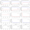 |
Fig. 2. Same as in Fig. 1 but for an initially anisotropic core Ac(0) ≃ Ah(0). |
| In the text | |
|
Fig. 3. Linear WI thresholds and QL dynamical paths of temperature anisotropy Ah, c derived for uh = 0.0, are compared with the quasi-stable states of electron halo (left) and core (right) populations from slow winds (VSW < 500 km s−1). |
| In the text | |
|
Fig. 4. Linear WI thresholds and QL dynamical paths of temperature anisotropy Ah, c derived for uh = 0.25 (top) and 0.5 (bottom) compared with the quasi-stable states of the electron halo (left) and core (right) populations from fast winds (VSW > 500 km s−1). |
| In the text | |
Current usage metrics show cumulative count of Article Views (full-text article views including HTML views, PDF and ePub downloads, according to the available data) and Abstracts Views on Vision4Press platform.
Data correspond to usage on the plateform after 2015. The current usage metrics is available 48-96 hours after online publication and is updated daily on week days.
Initial download of the metrics may take a while.