| Issue |
A&A
Volume 625, May 2019
|
|
|---|---|---|
| Article Number | A122 | |
| Number of page(s) | 16 | |
| Section | Catalogs and data | |
| DOI | https://doi.org/10.1051/0004-6361/201935368 | |
| Published online | 24 May 2019 | |
CIELO-RGS: a catalog of soft X-ray ionized emission lines⋆
1
SRON Netherlands Institute for Space Research, Sorbonnelaan 2, 3584 CA Utrecht, The Netherlands
e-mail: j.mao@sron.nl
2
Department of Physics, University of Strathclyde, G4 0NG Glasgow, UK
3
Leiden Observatory, Leiden University, PO Box 9513, 2300 RA Leiden, The Netherlands
4
ESA European Space Research and Technology Centre (ESTEC), Keplerlaan 1, 2201 AZ Noordwijk, The Netherlands
5
European Space Agency (ESA), European Space Astronomy Centre (ESAC), Villanueva de la Cañada, 28691 Madrid, Spain
6
Institut für Astronomie und Astrophysik, Universität Tübingen, Sand 1, 72076 Tübingen, Germany
Received:
26
February
2019
Accepted:
4
April
2019
Context. High-resolution X-ray spectroscopy has advanced our understanding of the hot Universe by revealing physical properties like kinematics, temperature, and abundances of the astrophysical plasmas. Despite technical and scientific achievements, the lack of scientific products at a level higher than count spectra is hampering complete scientific exploitation of high-quality data. This paper introduces the Catalog of Ionized Emission Lines Observed by the Reflection Grating Spectrometer (CIELO-RGS) onboard the XMM-Newton space observatory.
Aims. The CIELO-RGS catalog aims to facilitate the exploitation of emission features in the public RGS spectra archive. In particular, we aim to analyze the relationship between X-ray spectral diagnostics parameters and measurements at other wavelengths. This paper focuses on the methodology of catalog generation, describing the automated line-detection algorithm.
Methods. A moderate sample (∼2400 observations) of high-quality RGS spectra available at XMM-Newton Science Archive is used as our starting point. A list of potential emission lines is selected based on a multi-scale peak-detection algorithm in a uniform and automated way without prior assumption on the underlying astrophysical model. The candidate line list is validated via spectral fitting with simple continuum and line profile models. We also compare the catalog content with published literature results on a small number of exemplary sources.
Results. We generate a catalog of emission lines (1.2 × 10⁴) detected in ∼1600 observations toward stars, X-ray binaries, supernovae remnants, active galactic nuclei, and groups and clusters of galaxies. For each line, we report the observed wavelength, broadening, energy and photon flux, equivalent width, and so on.
Key words: X-rays: general / techniques: spectroscopic
The CIELO-RGS catalog is only available at the CDS via anonymous ftp to cdsarc.u-strasbg.fr (130.79.128.5) or via http://cdsarc.u-strasbg.fr/viz-bin/qcat?J/A+A/625/A122
© ESO 2019
1. Introduction
High-resolution X-ray spectroscopy has the potential to reveal the physics of the plasma state that accounts for much of the material in the observable universe. The X-ray band contains the inner-shell transitions of all abundant elements from C through N, O, Ne, Mg, Si, S, Ca, Fe and Ni. X-ray spectra of cosmic sources typically consist of a mixture of ionic or atomic emission or absorption lines and electron continuum components. Observed spectra can be modeled in order to identify the underlying physics and dynamics of the plasma concerned. They often depart from the ideal conditions of equilibrium and spatial uniformity. It is not coincidental that the availability of high-resolution data in the X-ray domain at the beginning of the current millennium has triggered important developments in the modeling of X-ray emitting plasma (Behar et al. 2001; Hitomi Collaboration 2018), in the collisionally ionized as well as in the photo-ionized regime.
A giant leap in this field was achieved with the launch of Chandra and XMM-Newton carrying high-sensitivity, high-resolution grating systems. In particular, the Reflection Grating Spectrometer (RGS; den Herder et al. 2001) on board XMM-Newton (Jansen et al. 2001) consists of an array of reflection gratings that diffract the light focused by two of the X-ray telescopes to an array of dedicated charge-coupled device detectors (CCDs). The RGS achieves high resolving power (150 to 800) over an energy range from 0.35 to 2 keV (≃6 to 35 Å, in the first spectral order). Thanks to the unprecedented collecting area of the XMM-Newton telescopes, the RGS is the most sensitive high-resolution X-ray detector currently in operation. Its performance and excellent calibration quality (de Vries et al. 2015) have allowed for breakthrough advancements in astrophysical fields as diverse as cool and active stars, X-ray binaries, galaxy clusters, and active galactic nuclei (AGNs), to mention just a few (Kahn et al. 2002).
Despite these outstanding technical and scientific achievements, complete scientific exploitation of the plasma diagnostic information enclosed in RGS spectroscopic data is still partly hampered by the lack of scientific products at a level higher than count spectra. Astronomers interested in extracting plasma diagnostics from RGS spectra must analyze them through the a forward-folding technique, which requires specialized software and can be potentially cumbersome when applied to spectra with good signal-to-noise ratios.
This paper describes CIELO-RGS1 (“CIELO” hereafter), a catalog of emission lines detected by the RGS instrument over more than 15 years of XMM-Newton science operations. To our knowledge CIELO is the first published catalog of its kind in high-energy astrophysics. The paper is organized as follows. Section 2 describes the procedure followed to reduce and select the optimal sample of RGS spectra from which the CIELO catalog has been produced. Section 3 describes the algorithm employed to select a sample of candidate emission lines on each RGS spectrum, later validated through spectral fitting. The catalog structure is described in Sect. 4. A selection of preliminary science results from the catalog as a whole is presented in Sect. 5, followed by our conclusions in Sect. 6. Future papers will discuss the application of CIELO to a wide range of astrophysical contexts and problems.
The CIELO catalog, data, and source codes used for creating the figures in this paper can be found at Zenodo2.
2. Spectra selection and reduction
The CIELO catalog is based on a subset of the RGS spectra available in the XMM-Newton Science Archive (XSA).
This subset has been taken from the work of Bensch et al. (2014). These authors examined all the RGS data available as of 1 December 2014 in order to identify those that are scientifically useful.
The method devised was based on two properties: an estimation of the signal-to-noise ratio of the spectrum, for which a minimum value of 10 was required, and a spatial profile of the spectrum along the cross-dispersion direction of the spectral image. This profile was fitted with a Gaussian function. For the spectrum to be considered useful, the fitting parameters needed to be well determined and within some pre-defined range (e.g., the width of the fitted Gaussian could not be narrower than the instrumental spatial resolution, and the maximum had to be close to the center of the field-of-view).
Out of the 8500 observations studied, 5000 (59%) passed these two acceptance criteria. These 5000 observations were further sub-divided into two categories: “Top quality” observations for which both RGS 1 and RGS 2 spectra were selected (28% of the initial sample), and “Good” observations, with only RGS 1 or RGS 2 considered as useful (31% of the initial sample). The sample used here is composed of the 2421 observations classified as Top quality in Bensch et al. (2014).
The data used in this work were taken from the XMM-Newton Science Archive (XSA). For each of the selected observations, the following data were downloaded: extracted first- order total (i.e., source+background) spectra, extracted first-order background spectra, and first-order response matrices (those for RGS also include the effective area), for RGS 1 and RGS 2.
These data were obtained from the raw observation data file (ODF) after automatic processing with the pipeline processing system (PPS). The PPS extracts RGS source spectra using the coordinates given in the original observational proposal, and an extraction region with a spatial size of 95% of the cross-dispersion PSF. The background is extracted from the region between 98% and 100% of the cross-dispersion PSF. A region including 95% of the pulse-height distribution is used in the extraction of both source and background spectra.
3. Catalog generation
Sophisticated plasma models are widely used for detailed analysis of emission features in high-resolution X-ray spectra (e.g., Broersen et al. 2011; Gu et al. 2016; Mao et al. 2018, 2019). While this approach yields self-consistent physical interpretations (e.g., temperature, density, and abundance) of the spectral features, it requires extensive prior knowledge of the source of interest, including but not limited to the cosmological redshift, line-of-sight galactic absorption, which and how many plasma models to use (collisional ionized, photoionized, non-equilibrium ionization, and charge exchange), and sometimes a multi-component model of the continuum. This approach is not applicable for the analysis of a large sample like CIELO-RGS.
An alternative approach is to use a phenomenological fit (e.g., Guainazzi & Bianchi 2007; Pinto et al. 2016; Psaradaki et al. 2018) for individual emission features. Typically, the (local) continuum is simply modeled as a (local) power law or spline function. Subsequently, it is common for the investigators to identify the emission features by eye or to scan the spectrum using a Gaussian/delta profile. Each emission feature is then modeled with a delta function or a Gaussian function with fixed width.
The phenomenological analysis is straightforward. It requires no prior knowledge of the source if all the emission lines are narrow and unresolved. When the emission lines are broader than the spectral resolution of the instrument, assuming that all the emission features have identical broadening, then the only prior knowledge needed is that of the line broadening.
The above issue with conventional phenomenological analysis is tractable with a line-detection algorithm based on wavelet transform. We note that wavelet transform analyses have proven to be suitable for both spectral and imaging analysis in astronomy (e.g., Bury et al. 1996; Starck et al. 1997; Machado et al. 2013). In particular, the concept of the multi-scale peak detection (MSPD) initially proposed in the chemistry community Zhang et al. (2015, Z15 hereafter) was followed for the present work.
The advantage of MSPD is that it extracts information from high-throughput spectra in a rapid way without any prior knowledge. Strong and weak, broad and narrow, symmetric and asymmetric spectral features on top of a continuum can be easily detected (Sect. 3.1). Once the number of significant spectral features is determined, the aforementioned phenomenological fit can be performed in a uniform and automated way (Sect. 3.2).
We should point out that the original MSPD algorithm shown in Z15 needs to be tailored for RGS data analysis. Z15 took advantage of “ridges” (local maxima, explained in Sect. 3.1), “valleys” (local minima) and “zero-crossings” (sign changes) for the peak detection. As MSPD does not estimate/fit the continuum, the presence of continuum breaks in the RGS spectra (e.g., CCD gaps) would lead to artificial “valleys” and “zero-crossings”. Furthermore, in Z15, the signal and noise levels are defined as the maximum and the 90th percentile within a selected window for each potential peak3. This would not work properly for closely located emission features, such as for example He-like triplets in many astrophysical spectra.
3.1. Multi-scale peak detection
The present MSPD algorithm flows as follows. It is based on the continuous wavelet transform (CWT) using the Mexican hat wavelet (or Ricker wavelet)
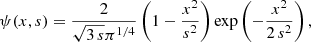
where x is the number of points used to describe the wavelet and s is the scale of the wavelet. Figure 1 shows an example of the Mexican hat wavelet at some scales.
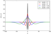 |
Fig. 1. Mexican hat wavelet at different scales. Here we use 201 points (i.e., 200 bins) to describe the wavelet. The corresponding Y-value is placed at the center of the each bin to mimic the real spectra. |
The input spectrum S(N) is convolved with a set of wavelet functions ψ(N′, s), where N′ is the minimum value between the number of bins (N) in the input spectrum and ten times the scale (10 × s) and the scale (s) ranges from 1 to 50. The top panel of Fig. 2 shows the observed RGS flux spectrum of NGC 1068 (ObsID: 0111200101) in the 6−8 Å wavelength range (∼3200 spectral bins). The second panel of Fig. 2 presents the results of the continuous wavelet transform (CWT) with s = 3 in blue and 37 in orange, respectively. Peaks appear in the observed spectrum yield larger CWT coefficients. The third panel of Fig. 2 presents the color-coded CWT coefficients. This can be viewed as the dilation and translation of peaks. The redder (larger) the coefficient, the more prominent the peak. Ridges are introduced as curves of local maxima in the 2D wavelet space, where the rows and columns are scales and bins, respectively. The bottom panel of Fig. 2 illustrates ridges across different scales for NGC 1068. Ridges are denser at smaller scales as the spectrum is nosier.
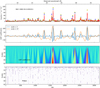 |
Fig. 2. Top panel: observed RGS flux spectrum of NGC 1068 (ObsID: 0111200101). The RGS 1 and RGS 2 spectra (in red) are combined. Error bars are not shown for clarity. The blue triangles mark peaks detected by the MSPD algorithm (Zhang et al. 2015) with (their definition of) signal-to-noise ratio ≥7. The yellow circles mark peaks detected by the present work at a significance level of ≳2.7σ. The estimated continuum in green is based on the asymmetrically reweighted penalized least squares algorithm (arPLS, Baek et al. 2015). The estimated continuum is shown merely for guidance as it is independent of the MSPD algorithm. The second panel gives the coefficients (Y-axis) of the continuous wavelet transform (CWT) of the spectrum at scale = 3 (blue) and 37 (orange). The third panel is a color map of the CWT coefficients at different scales (Y-axis) and at each spectral bin (X-axis). The redder the color, the larger the CWT coefficient. The bottom panel presents the so-called ridges across different scales. |
A ridge in the wavelet space does not necessarily correspond to a prominent emission feature in the observed spectrum (e.g., Fig. 3). Starting from the left-hand side of the 2D wavelet space (i.e., shorter observed wavelength), for each ridge, we track the bin numbers and CWT coefficients from the largest scale present down to s = 2. We note that a ridge starting from a larger scale might diverge into two or more ridges at smaller scales due to the presence of noise. Therefore, we stop tracking the ridges at s = 2. The ridge of a potential line should meet the following empirical criteria:
-
1.
Local maxima should appear at larger scales s ≳ 6;
-
2.
At least 20% of bin numbers should be identical so that the ridge is relatively straight;
-
3.
The maximum CWT coefficient should be at least 2.7σ above the average.
The quoted numbers are used for the present sample analysis, which can certainly be fine tuned for a case study. The wavelength corresponds to the bin number appearing in most scales of the selected ridge that is assigned to the potential line. This choice of wavelength is arbitrary but not critical because it will be determined more accurately via spectral fitting (Sect. 3.2).
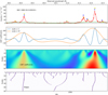 |
Fig. 3. Similar to Fig. 2 but in the neighborhood of the O VIII Lyα line and the O VII He-like triplets. |
While the present MSPD algorithm successfully detects the majority of visible peaks (by eye) in the point-like source NGC 1068, we need to validate its performance on extended sources. Since the RGS spectrometer is slitless, the emission line profiles of extended sources would appear broader, which complicates the analysis in practise. Figure 4 shows the application of the present MSPD algorithm to the observed flux spectrum of NGC 5044 (ObsID: 0554680101). Again, the majority of visible peaks (by eye) are detected. Meanwhile, the relatively poorer signal-to-noise of the spectrum leads to more false detections. These false peaks are filtered out after the following spectral fitting.
3.2. Spectral fitting
The first-order background subtracted RGS 1 and RGS 2 spectra, as well as response matrices, are converted into the SPEX (Kaastra et al. 1996, 2018) format through the SPEX task trafo. For each observation, RGS 1 and RGS 2 spectra, if available, are fitted simultaneously. About 1% of the observations in the BIRD catalog have either only RGS 1 or RGS 2 data, which are also fitted with the data available.
The full-width-half-maximum (FWHMinst) of the first-order RGS instruments is ∼0.06−0.09 Å4. For extended sources, due to the spatial broadening (θ ≥ 0.8 arcmin or 90% of the point-spread-function) along the cross-dispersion direction, the effective FWHMeff is bigger than the instrumental FWHMinst,
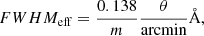
where m is the spectral order (Tamura et al. 2004) and, in our case, m = 1.
The default bin size of the RGS spectra is 0.01 Å, which is clearly over-sampling. Therefore, we re-bin each RGS spectrum to achieve optimal binning (Kaastra & Bleeker 2016), which is one half to one third of the maximum between FWHMinst and FWHMeff. That is to say, in any case, the minimum binning factor is 3.
Wavelength and flux values in CIELO are observed measurements. We did not apply any corrections for redshift or for X-ray absorption.
For each spectrum, the continuum is modeled with a spline function, which consists of a grid of nine points evenly distributed in the 6−38 Å wavelength range. The spline continuum modeling has been used successfully in for example Kaastra et al. (2011).
Without any prior knowledge of the astrophysical properties of the targets, all emission features are modeled with Gaussian profiles. The multi-scale peak-detection algorithm (Sect. 3.1) provides the number of emission features to SPEX, as well as the initial guess of the wavelength of each feature. The normalization, wavelength, and broadening of each Gaussian are free to vary during the fit. We note that the velocity broadening of each Gaussian is constrained to be 0−104 km s−1. The upper limit is set to cover broad emission features from the broad-line region in AGNs (Blandford et al. 1990).
The optimization method used here is the classical “Levenberg-Marquardt” method, which might not lead to the global minimum. A better fit can be found during the error search of the parameters for each Gaussian. If so, we refit the spectrum starting from those values that lead to better (or lower) statistics. We stop the iteration if the improvement on the ΔC ≲ 0.5, and limit the number of iterations (≤5) if the convergence is slow. The slow convergence is partly due to those very broad emission features, where the broadening and the normalization parameters are degenerate to some extent.
The best-fit parameters of an emission line are included in the final catalog if its normalization is above zero at a 3σ confidence level and the energy flux is ≳10−18 W m−2.
4. Catalog structure
The CIELO catalog is in the form of a machine readable ASCII table and a FITS table. Both tables consist of 10981 rows from 1492 unique observations and 16 columns: Col. (1) is the ObsID; Cols. (2)−(4) are the wavelength (in Å) and the 1σ lower and upper limits; Cols. (5)−(7) are the FWHM in Å and the 1σ lower and upper limits; Cols. (8)−(10) are normalization (in 1044 ph s−1) and the 1σ lower and upper limits; Col. (11) is the observed energy flux (in W m−2); Col. (12) is the observed photon flux (in ph m−2 s−1); Col. (13) is the modeled (spline) continuum photon flux density at the line center (in ph m−2 s−1 Å−1), and Col. (14) is the equivalent width (EW in Å) defined as follows:

where Fline is the observed photon flux of the line (Col. 12) and Fcont is the modeled (spline) continuum photon flux density at the line center (Col. 13). The last two columns are the redshift (from Simbad, Col. 15) and target name (from XSA, Col. 16).
5. Results
CIELO includes data from ∼66% of the BIRD “top quality” observations. The targets of the remaining observations include some pulsars, BL-Lac objects, gamma-ray bursts, voids, and so on. The soft X-ray spectra of these targets are featureless with small uncertainties on the (continuum) flux.
Figure 5 gives an overview of the observed wavelength distribution of all the lines included in the catalog. H-like Lyman series, He-like triplets, and Ne-like Fe XVII resonance, and forbidden lines dominate the catalog. Since observations are biased to nearby and bright targets, the observed wavelength of the emission lines peaks around the corresponding rest frame wavelength.
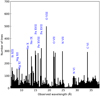 |
Fig. 5. Histogram of the CIELO catalog as a function of observed wavelength. The rest frame wavelength of H-like Lyα and He-like resonances lines are labeled for guidance. |
Here we present comparisons of our results with published literature results. The comparisons are limited to point-like sources. As for extended sources like groups and clusters of galaxies (e.g., Kaastra et al. 2001; Tamura et al. 2001; Werner et al. 2006) and supernovae remnants (e.g., Rasmussen et al. 2001; van der Heyden et al. 2003; Broersen et al. 2011), results of plasma modeling (e.g., temperature, abundance, emission measure) are usually provided, instead of a list of emission lines.
5.1. Local obscured AGN: NGC 1068
NGC 1068 is the prototypical Seyfert 2 galaxy in the local Universe with a redshift of z = 0.0038 (Huchra et al. 1999). Here we take the RGS spectrum of NGC 1068 (ObsID: 0111200101, 41 ks effective exposure) as an example for local obscured AGNs. We show in Fig. 6 a comparison of the emission lines detected in the present study and Kinkhabwala et al. (2002, K02 hereafter). More details can be found in Table A.1. We also show in Fig. A.1 the results of spectral fitting (Sect. 3.2).
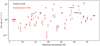 |
Fig. 6. Emission lines detected in the RGS spectrum of NGC 1068 during the present study (black) and by Kinkhabwala et al. (2002, red). For visibility, for each data point we assign the line width (in Å instead of the wavelength uncertainty) to the horizontal error bar. |
K02 reported measurements of 40 lines and six RRC in their Tables 1 and 2, respectively. The CIELO catalog contains 38 lines (including RRC). The difference in the total number of lines is not unexpected. The present analysis does not benefit from prior knowledge of the atomic origin of the emission features. Consequently, the resonance and intercombination lines of Ne IX, for example, are fitted as two lines in K02, yet as one line (i.e., a single Gaussian profile) here; the O VIII Lyγ and putative Fe XXIV, Ar XI, and S XII lines are missed in K02 but are included here. Moreover, the present work is designed (Sect. 3.1) to omit relatively weak lines. Accordingly, weak lines like the O VIII Lyδ line are included in K02 but are missed here.
If lines are well separated, the velocity shifts (voff) and broadening (σv), and the observed photon fluxes (Fpho) from the above two analyses are consistent with each other. The Ne X Lyα line is an exception, where the observed wavelength and velocity broadening are (12.180 ± 0.004) Å and 470 ± 120 km s−1 in K02 yet (12.206 ± 0.005) Å and 1200 ± 160 km s−1 in the present work. The observed Ne X Lyα line profile shown in Fig. A.1 deviates to a Gaussian profile, which leads to the measurement bias. We also note that 12.165 Å and  km s−1 are quoted by Kallman et al. (2014, K14 hereafter), where the spectral analysis is based on the 450 ks Chandra high-energy transmission grating spectroscopy data.
If lines are blended with each other, disagreement on the velocity shift and broadening are expected. The Ne IX He-like triplets around 13.5 Å is a typical example. We note that both the present work and K14 cannot distinguish the resonance from the intercombination lines.
Furthermore, at shorter wavelengths (λ ≲ 20 Å), the line widths obtained in the present work are in general larger than those given in K02, but within the upper limits given by K14. Better agreement is found at longer wavelengths (λ ≳ 20 Å).
There are two caveats in Table A.1. First, K02 assign a single value of 6.69 Å to the rest-frame wavelength of the Si XIII He-like triplets. The wavelengths of the resonance, intercombination, and forbidden lines are 6.648 Å (w), 6.685 Å (x), 6.688 Å (y), and 6.739 Å (z), respectively. Second, the present work fails to properly interpret the intercombination lines (x and y) of N VI around 29 Å. The line profile has a single peak in RGS 1 but a double peak in RGS 2 (the fourth panel of Fig. A.1). This leads to significantly biased results. K02 tied the velocity broadening of the He-like triplets and yielded more proper results.
5.2. Stars: Procyon and HD 159176
High-quality RGS spectra of various active stars are available. We take Procyon and HD 159176 as two examples to illustrate results from the present analysis.
The X-ray spectrum of Procyon is dominated by the late-type (F5 IV-V) optically bright star (with a faint white dwarf companion). The stellar corona has a temperature of ∼(1−3) × 106 K and exhibits a cooler X-ray spectrum than magnetically active stars (Raassen et al. 2002, R02 hereafter). In Fig. 7, we compare the observed wavelengths and fluxes of ObsID 0123940101 (45.2 ks effective exposure) with those from Table 1 of R02, where both RGS and LEGS results are available. More details can be found in Table A.2. We also show in Fig. A.2 the results of spectral fitting (Sect. 3.2).
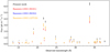 |
Fig. 7. Emission lines detected in the RGS spectrum of Procyon during the present study (black) and Raassen et al. (2002, red for RGS 1, blue for RGS 2, and orange for LETGS). The wavelength uncertainty is not visible here. |
Apart from those lines that we fail to individually identify here (e.g., around 13.56 Å and 36.45 Å), a good agreement can be found between the present work and R02 in terms of the observed wavelength. As for the line (photon) fluxes, we find larger values in the present work in addition to only a few consistent results (e.g., the O VIII 18.628 line). This is mainly due to the two different approaches for the continuum. As described in Sect. 3.2, a spline function is used here for the global continuum. On the other hand, R02 adopted a constant local “background” level. The local background was adjusted for each emission line to account for the real continuum and the pseudo-continuum created by the overlap of several neglected weak lines.
Unlike the narrow and “regular” emission lines in Procyon, the emission lines in HD 159176 are rather broad and asymmetric (neither Gaussian nor Lorentzian). HD 159176 is a double-lined spectroscopic binary (O7V + O7V) in the young open cluster NGC 6383 (Trumpler 1930). As can be seen in Fig. A.3, the Gaussian profiles adopted in the present analysis manage to capture the main features yet fail to account for the details. We also note that fitting RGS 1 and RGS 2 simultaneously rejects those features that appear in only one of the instruments (e.g., around ∼10 Å) and those features that appear only in one instrument (e.g., the one around ∼9.3 Å).
According to De Becker et al. (2004), the O VIII Lyα line has an estimated FWHM of 2500 km s−1. Moreover, it is slightly blue-shifted ∼300−600 km s−1, though the highest peak in the profile is found near the rest frame wavelength 18.967 Å (De Becker et al. 2004). The present analysis yields an FWHM of (0.130 ± 0.014) Å, i.e., (2060 ± 220) km s−1 and an observed wavelength of (18.975 ± 0.008) Å, that is, blue-shifted by (130 ± 120) km s−1. Given the complicated nature of this spectrum, our results are acceptable.
5.3. X-ray binaries: Her X-1
Her X-1 is a bright intermediate-mass X-ray binary (Schreier et al. 1972) exhibiting an unusual long-term X-ray flux modulation with a period of 35 days (Giacconi et al. 1973). The 35-day X-ray light curve is asymmetric and contains two peaks: a state of eight-day duration reaching the peak flux Fmax named the main-on state and a four-day duration reaching one third of the maximum named the short-on state. The rest is named the low state with flux twenty times lower than the maximum (Jimenez-Garate et al. 2002, JG02).
We inspect the RGS spectra of Her X-1 at three different orbital phases: 0134120101 (main), 0111060101 (low), and 0111061201 (short-on). Figure 8 visualizes the comparison of emission lines reported in the present work and JG02. Tabulated results are given in Table A.3. The plot of the spectral fitting for the short-on phase can be found in Fig. A.4.
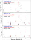 |
Fig. 8. Comparison of emission lines detected in the RGS spectra of Her X-1 in three different orbital phases. The present work and Jimenez-Garate et al. (2002) are shown in black and red, respectively. |
Minor differences are found between the present analysis and JG02. The present work does not include the weak resonance line in the O VII He-like triplets. The N VII Lyα line is found to be rather broad (4200 ± 1600) km s−1 in the present work. The width was fixed to 3200 km s−1 in JG02, based on their width of O VII He-like triplets. As a result, the line (photon) flux reported here is slightly higher (at a 2σ confidence level) than that of JG02.
Moreover, we also include a few broad features at 6.4 Å, 6.7 Å, and 14.1 Å. Such broad features are likely due to calibration uncertainties of the instrument. The smaller the statistical uncertainty, the more prominent such systematic uncertainties.
5.4. Comparison of plasma diagnostics: stars vs. obscured AGNs
The intensity of the brightest components of n = 2 to n = 1 transitions in He-like ions can be combined into ratios with a strong diagnostic power of the electron density [R(ne)] and electronic temperature [G(Te)] (Gabriel & Jordan 1969):

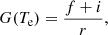
where f, i, and r are the intensities of the forbidden (z; 1s2 1S0 – 1s2s 3S1), intercombination (x,y; 1s21S0 – 1s2p 3P2, 1), and resonance (w; 1s21S0 – 1s2p 1P1) lines, respectively. The same diagnostic ratios can be used to study photoionised plasma as well (Porter & Ferland 2007). Indeed, they can be used to identify the dominant ionization mechanism (Porquet & Dubau 2000).
The CIELO catalog allows for studies of these diagnostic parameters on large source populations. As an example, in Fig. 9 we show the R versus G diagnostic plot for the OVII He-α transition derived from the CIELO catalog for the two soft, X-ray brightest, heavily obscured AGNs (NGC 1068, and NGC 4151) (Guainazzi & Bianchi 2007), and for a sample of active stars. Multiple data points for each source correspond to different observations. The AGN X-ray spectra are dominated by plasma photoionized by the intense radiation field of the active nucleus (Kinkhabwala et al. 2002), most likely due to X-ray diffuse emission associated with the extended narrow line regions (Bianchi et al. 2006). The variability of the R parameter reflects time changes in the ratio between the forbidden and the intercombination component that could be related to the UV illumination of the ionized nebula in a radiation-driven wind (Landt et al. 2015). Stellar spectra should be instead dominated by optically thin collisionally ionized plasma. The CIELO diagnostic diagram nicely separates the two classes, as expected.
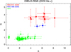 |
Fig. 9. OVII He-α diagnostic parameters R and G for the two brightest heavily obscured AGNs (NGC 1068, blue; NGC 4151, red), and for a sample of active stars (green) in CIELO-RGS. |
6. Summary
In this paper we present CIELO-RGS, the first systematic catalog of emission lines detected by the RGS instrument (den Herder et al. 2001) on-board XMM-Newton. CIELO-RGS was built using high-quality spectra accumulated during more than 5000 observations performed over 15 years of XMM-Newton science operations. This catalog is intended to be an additional tool to facilitate the exploitation of the RGS spectra available in the public science archive, and in particular for comparisons of X-ray spectral diagnostic parameters and measurements at other wavelengths.
The catalog generation is based on a two-tier process. First, each RGS spectrum was analyzed searching for candidate emission lines with a technique fully independent of the spectral modeling, and therefore in principle of the intrinsic physical and astrophysical nature of the emitting plasma. This technique is one version of a multi-scale peak-detection algorithm, robustly tested in other scientific contexts (Z15). This step provides a list of candidate emission lines detected in each individual observation spectrum over the appropriate range of frequency scales (upper-bound by the instrumental resolution). This list of candidate emission lines is subsequently validated through a formal forward-folding spectral fitting process that properly takes into account the instrumental transfer function, the observation background, and the rigorous statistical conditions for spectral binning (Kaastra & Bleeker 2016). The resulting catalog includes the following measured observable for each line: wavelength, intrinsic profile width, normalization, energy and photon flux, and equivalent width, as well as a phenomenological parameterization of the underlying continuum.
In this paper we present some illustrative examples of the wide range of scientific themes that such a catalog can address, such as the ionization mechanism and dynamics of the extended narrow line region in AGNs, plasma diagnostics in optically thin, collisionally ionised plasma in stars or the intra-cluster medium permeating galaxy clusters, and coronal emission in accreting stellar-mass black holes. These topics will be further developed in specific future papers.
Details can be found in the source code available at https://github.com/zmzhang/libPeak/blob/master/peak_detection.py
We refer readers to Fig. 82 of the XMM User’s hand book (available at https://xmm-tools.cosmos.esa.int/external/xmm_user_support/documentation/uhb/rgsresolve.html) for details.
Acknowledgments
We thank the referee for careful reading of the manuscript. The authors gratefully acknowledge a generous financial support by the Divisional Funding of the Science Support Office at ESA, in the framework of the EXPRO contract 40000124950/18/NL/JB/gg. J. M. acknowledges discussions and consultations with J. de Plaa, N. Loiseau, M. Mehdipour, and C. de Vries. JM is supported by STFC (UK) through the University of Strathclyde UK APAP network grant ST/R000743/1. SRON is supported financially by NWO, the Netherlands Organization for Scientific Research.
References
- Baek, S.-J., Park, A., Ahn, Y.-J., & Choo, J. 2015, Analyst, 140, 250 [NASA ADS] [CrossRef] [Google Scholar]
- Behar, E., Sako, M., & Kahn, S. M. 2001, ApJ, 563, 497 [NASA ADS] [CrossRef] [Google Scholar]
- Bensch, K., Santos-Lleo, M., & Gonzalez-Riestra, R. 2014, The X-ray Universe 2014, 36 [Google Scholar]
- Bianchi, S., Guainazzi, M., & Chiaberge, M. 2006, A&A, 448, 499 [NASA ADS] [CrossRef] [EDP Sciences] [Google Scholar]
- Blandford, R. D., Netzer, H., Woltjer, L., Courvoisier, T. J. L., & Mayor, M. 1990, Active Galactic Nuclei (New York: Springer-Verlag Berlin Heidelberg), 97 [Google Scholar]
- Broersen, S., Vink, J., Kaastra, J., & Raymond, J. 2011, A&A, 535, A11 [NASA ADS] [CrossRef] [EDP Sciences] [Google Scholar]
- Bury, P., Ennode, N., Petit, J.-M., et al. 1996, NIMPA, 383, 572 [NASA ADS] [CrossRef] [Google Scholar]
- De Becker, M., Rauw, G., Pittard, J. M., et al. 2004, A&A, 416, 221 [NASA ADS] [CrossRef] [EDP Sciences] [Google Scholar]
- den Herder, J. W., Brinkman, A. C., Kahn, S. M., et al. 2001, A&A, 365, L7 [NASA ADS] [CrossRef] [EDP Sciences] [Google Scholar]
- de Vries, C. P., den Herder, J. W., Gabriel, C., et al. 2015, A&A, 573, A128 [NASA ADS] [CrossRef] [EDP Sciences] [Google Scholar]
- Gabriel, A. H., & Jordan, C. 1969, Nature, 221, 947 [NASA ADS] [CrossRef] [Google Scholar]
- Giacconi, R., Gursky, H., Kellogg, E., et al. 1973, ApJ, 184, 227 [NASA ADS] [CrossRef] [Google Scholar]
- Gu, L., Kaastra, J., & Raassen, A. J. J. 2016, A&A, 588, A52 [NASA ADS] [CrossRef] [EDP Sciences] [Google Scholar]
- Guainazzi, M., & Bianchi, S. 2007, MNRAS, 374, 1290 [NASA ADS] [CrossRef] [Google Scholar]
- Hitomi Collaboration (Aharonian, F., et al.) 2018, PASJ, 70, 12 [NASA ADS] [Google Scholar]
- Huchra, J. P., Vogeley, M. S., & Geller, M. J. 1999, ApJS, 121, 287 [NASA ADS] [CrossRef] [Google Scholar]
- Jansen, F., Lumb, D., Altieri, B., et al. 2001, A&A, 365, L1 [NASA ADS] [CrossRef] [EDP Sciences] [Google Scholar]
- Jimenez-Garate, M. A., Hailey, C. J., den Herder, J. W., Zane, S., & Ramsay, G. 2002, ApJ, 578, 391 [NASA ADS] [CrossRef] [Google Scholar]
- Kaastra, J. S. 2017, A&A, 605, A51 [NASA ADS] [CrossRef] [EDP Sciences] [Google Scholar]
- Kaastra, J. S., & Bleeker, J. A. M. 2016, A&A, 587, A151 [NASA ADS] [CrossRef] [EDP Sciences] [Google Scholar]
- Kaastra, J. S., Mewe, R., & Nieuwenhuijzen, H. 1996, UV and X-ray Spectroscopy of Astrophysical and Laboratory Plasmas (Tokyo: Univ. Ac. Press), 411 [Google Scholar]
- Kaastra, J. S., Ferrigno, C., Tamura, T., et al. 2001, A&A, 365, L99 [NASA ADS] [CrossRef] [EDP Sciences] [Google Scholar]
- Kaastra, J. S., Steenbrugge, K. C., Detmers, R. G., et al. 2011, A&A, 534, A38 [NASA ADS] [CrossRef] [EDP Sciences] [Google Scholar]
- Kaastra, J. S., Raassen, A. J. J., de Plaa, J., & Gu, L. 2018, SPEX X-ray Spectral Fitting Package (Version 3.05.00). Zenodo, DOI: 10.5281/zenodo.2419563 [Google Scholar]
- Kahn, S. M., Behar, E., Kinkhabwala, A., & Savin, D. W. 2002, RSPTA, 360, 1923 [NASA ADS] [CrossRef] [Google Scholar]
- Kallman, T., Evans, D. A., Marshall, H., et al. 2014, ApJ, 780, 121 [NASA ADS] [CrossRef] [Google Scholar]
- Kinkhabwala, A., Sako, M., Behar, E., et al. 2002, ApJ, 575, 732 [NASA ADS] [CrossRef] [Google Scholar]
- Landt, H., Ward, M. J., Steenbrugge, K. C., & Ferland, G. J. 2015, MNRAS, 449, 3795 [NASA ADS] [CrossRef] [Google Scholar]
- Machado, D. P., Leonard, A., Starck, J.-L., Abdalla, F. B., & Jouvel, S. 2013, A&A, 560, A83 [NASA ADS] [CrossRef] [EDP Sciences] [Google Scholar]
- Mao, J., Kaastra, J. S., Mehdipour, M., et al. 2018, A&A, 612, A18 [NASA ADS] [CrossRef] [EDP Sciences] [Google Scholar]
- Mao, J., de Plaa, J., Kaastra, J. S., et al. 2019, A&A, 621, A9 [NASA ADS] [CrossRef] [EDP Sciences] [Google Scholar]
- Pinto, C., Middleton, M. J., & Fabian, A. C. 2016, Nature, 533, 64 [NASA ADS] [CrossRef] [Google Scholar]
- Porquet, D., & Dubau, J. 2000, A&AS, 143, 495 [NASA ADS] [CrossRef] [EDP Sciences] [Google Scholar]
- Porter, R. L., & Ferland, G. J. 2007, ApJ, 664, 586 [NASA ADS] [CrossRef] [Google Scholar]
- Psaradaki, I., Costantini, E., Mehdipour, M., & Díaz Trigo, M. 2018, A&A, 620, A129 [NASA ADS] [CrossRef] [EDP Sciences] [Google Scholar]
- Raassen, A. J. J., Mewe, R., Audard, M., et al. 2002, A&A, 389, 228 [NASA ADS] [CrossRef] [EDP Sciences] [Google Scholar]
- Rasmussen, A. P., Behar, E., Kahn, S. M., den Herder, J. W., & van der Heyden, K. 2001, A&A, 365, L231 [NASA ADS] [CrossRef] [EDP Sciences] [Google Scholar]
- Schreier, E., Levinson, R., Gursky, H., et al. 1972, ApJ, 172, L79 [NASA ADS] [CrossRef] [Google Scholar]
- Starck, J.-L., Siebenmorgen, R., & Gredel, R. 1997, ApJ, 482, 1011 [NASA ADS] [CrossRef] [Google Scholar]
- Tamura, T., Kaastra, J. S., Peterson, J. R., et al. 2001, A&A, 365, L87 [NASA ADS] [CrossRef] [EDP Sciences] [Google Scholar]
- Tamura, T., Kaastra, J. S., den Herder, J. W. A., Bleeker, J. A. M., & Peterson, J. R. 2004, A&A, 420, 135 [NASA ADS] [CrossRef] [EDP Sciences] [Google Scholar]
- Trumpler, R. J. 1930, PASP, 42, 342 [NASA ADS] [CrossRef] [Google Scholar]
- van der Heyden, K. J., Bleeker, J. A. M., Kaastra, J. S., & Vink, J. 2003, A&A, 406, 141 [NASA ADS] [CrossRef] [EDP Sciences] [Google Scholar]
- Werner, N., Böhringer, H., Kaastra, J. S., et al. 2006, A&A, 459, 353 [NASA ADS] [CrossRef] [EDP Sciences] [Google Scholar]
- Zhang, Z.-M., Tong, X., Peng, Y., et al. 2015, Analyst, 140, 7955 [NASA ADS] [CrossRef] [Google Scholar]
Appendix A: Detailed comparisons of the examples
We show the best-fit models against the observed spectra for NGC 1068, Procyon, HD 15176, and Her X-1 in Sect. 5 (Figs. A.1–A.4). Comparisons of the emission lines among the present work and others are also shown (Tables A.1–A.3).
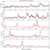 |
Fig. A.1. RGS spectrum of NGC 1068 (ObsID: 0111200101). RGS 1 and RGS 2 spectra are fitted simultaneously. RGS spectra are rebinned by a factor of 3. RGS 1 and RGS 2 data are shown in black and gray, respectively. The best-fit models are shown in red and pink for RGS 1 and RGS 2, respectively. The breaks (e.g., around 11.2 Å and 24 Å) are due to CCD gaps, bad pixels, etc. |
List of lines and radiative recombination continua (RRC) in NGC 1068.
List of lines in Procyon.
List of lines for Her X-1 at different orbital phases.
All Tables
All Figures
|
Fig. 1. Mexican hat wavelet at different scales. Here we use 201 points (i.e., 200 bins) to describe the wavelet. The corresponding Y-value is placed at the center of the each bin to mimic the real spectra. |
| In the text | |
|
Fig. 2. Top panel: observed RGS flux spectrum of NGC 1068 (ObsID: 0111200101). The RGS 1 and RGS 2 spectra (in red) are combined. Error bars are not shown for clarity. The blue triangles mark peaks detected by the MSPD algorithm (Zhang et al. 2015) with (their definition of) signal-to-noise ratio ≥7. The yellow circles mark peaks detected by the present work at a significance level of ≳2.7σ. The estimated continuum in green is based on the asymmetrically reweighted penalized least squares algorithm (arPLS, Baek et al. 2015). The estimated continuum is shown merely for guidance as it is independent of the MSPD algorithm. The second panel gives the coefficients (Y-axis) of the continuous wavelet transform (CWT) of the spectrum at scale = 3 (blue) and 37 (orange). The third panel is a color map of the CWT coefficients at different scales (Y-axis) and at each spectral bin (X-axis). The redder the color, the larger the CWT coefficient. The bottom panel presents the so-called ridges across different scales. |
| In the text | |
|
Fig. 3. Similar to Fig. 2 but in the neighborhood of the O VIII Lyα line and the O VII He-like triplets. |
| In the text | |
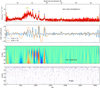 |
Fig. 4. Similar to Fig. 2 but for NGC 5044 (ObsID: 0554680101). |
| In the text | |
|
Fig. 5. Histogram of the CIELO catalog as a function of observed wavelength. The rest frame wavelength of H-like Lyα and He-like resonances lines are labeled for guidance. |
| In the text | |
|
Fig. 6. Emission lines detected in the RGS spectrum of NGC 1068 during the present study (black) and by Kinkhabwala et al. (2002, red). For visibility, for each data point we assign the line width (in Å instead of the wavelength uncertainty) to the horizontal error bar. |
| In the text | |
|
Fig. 7. Emission lines detected in the RGS spectrum of Procyon during the present study (black) and Raassen et al. (2002, red for RGS 1, blue for RGS 2, and orange for LETGS). The wavelength uncertainty is not visible here. |
| In the text | |
|
Fig. 8. Comparison of emission lines detected in the RGS spectra of Her X-1 in three different orbital phases. The present work and Jimenez-Garate et al. (2002) are shown in black and red, respectively. |
| In the text | |
|
Fig. 9. OVII He-α diagnostic parameters R and G for the two brightest heavily obscured AGNs (NGC 1068, blue; NGC 4151, red), and for a sample of active stars (green) in CIELO-RGS. |
| In the text | |
|
Fig. A.1. RGS spectrum of NGC 1068 (ObsID: 0111200101). RGS 1 and RGS 2 spectra are fitted simultaneously. RGS spectra are rebinned by a factor of 3. RGS 1 and RGS 2 data are shown in black and gray, respectively. The best-fit models are shown in red and pink for RGS 1 and RGS 2, respectively. The breaks (e.g., around 11.2 Å and 24 Å) are due to CCD gaps, bad pixels, etc. |
| In the text | |
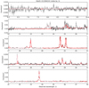 |
Fig. A.2. Similar to Fig. A.2 but for Procyon (ObsID: 0123940101). |
| In the text | |
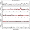 |
Fig. A.3. Similar to Fig. A.1 but for HD 159176 (ObsID: 0001730201). |
| In the text | |
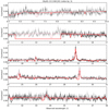 |
Fig. A.4. Similar to Fig. A.1 but for Her X-1 (ObsID: 0111061201). |
| In the text | |
Current usage metrics show cumulative count of Article Views (full-text article views including HTML views, PDF and ePub downloads, according to the available data) and Abstracts Views on Vision4Press platform.
Data correspond to usage on the plateform after 2015. The current usage metrics is available 48-96 hours after online publication and is updated daily on week days.
Initial download of the metrics may take a while.