| Issue |
A&A
Volume 624, April 2019
|
|
|---|---|---|
| Article Number | L1 | |
| Number of page(s) | 6 | |
| Section | Letters to the Editor | |
| DOI | https://doi.org/10.1051/0004-6361/201935105 | |
| Published online | 01 April 2019 | |
Letter to the Editor
Gaia DR2 reveals a star formation burst in the disc 2–3 Gyr ago
1
Dept. Física Quàntica i Astrofísica, Institut de Ciències del Cosmos, Universitat de Barcelona (IEEC-UB), Martí Franquès 1, 08028 Barcelona, Spain
e-mail: This email address is being protected from spambots. You need JavaScript enabled to view it.
2
Institut Utinam, CNRS UMR6213, Université de Bourgogne Franche-Comté, OSU THETA, Observatoire de Besançon, BP 1615, 25010 Besançon Cedex, France
3
Departamento de Física de la Tierra y Astrofísica, Facultad de Ciencias Físicas, Plaza Ciencias 1, Madrid 28040, Spain
Received:
22
January
2019
Accepted:
15
March
2019
Abstract
We use Gaia data release 2 (DR2) magnitudes, colours, and parallaxes for stars with G < 12 to explore a parameter space with 15 dimensions that simultaneously includes the initial mass function (IMF) and a non-parametric star formation history (SFH) for the Galactic disc. This inference is performed by combining the Besançon Galaxy Model fast approximate simulations (BGM FASt) and an approximate Bayesian computation algorithm. We find in Gaia DR2 data an imprint of a star formation burst 2–3 Gyr ago in the Galactic thin disc domain, and a present star formation rate (SFR) of ≈1 M⊙/yr. Our results show a decreasing trend of the SFR from 9–10 Gyr to 6–7 Gyr ago. This is consistent with the cosmological star formation quenching observed at redshifts z < 1.8. This decreasing trend is followed by a SFR enhancement starting at ∼5 Gyr ago and continuing until ∼1 Gyr ago which is detected with high statistical significance by discarding the null hypothesis of an exponential SFH with a p-value = 0.002. We estimate, from our best fit model, that about 50% of the mass used to generate stars, along the thin disc life, was expended in the period from 5 to 1 Gyr ago. The timescale and the amount of stellar mass generated during the SFR enhancement event lead us to hypothesise that its origin, currently under investigation, is not intrinsic to the disc. Thus, an external perturbation is needed for its explanation. Additionally, for the thin disc we find a slope of the IMF of α3 ≈ 2 for masses M > 1.53 M⊙ and α2 ≈ 1.3 for the mass range between 0.5 and 1.53 M⊙. This is the first time that we consider a non-parametric SFH for the thin disc in the Besançon Galaxy Model. This new step, together with the capabilities of the Gaia DR2 parallaxes to break degeneracies between different stellar populations, allow us to better constrain the SFH and the IMF.
Key words: Galaxy: evolution / Galaxy: disk / Galaxy: stellar content / Hertzsprung-Russell and C-M diagrams / stars: luminosity function / mass function / galaxies: interactions
© ESO 2019
1. Introduction
The star formation history (SFH) of the Milky Way disc contains essential information to understand the Galactic structure and evolution, including key information of its merger history (e.g. Gilmore 2001). Recently, Antoja et al. (2018) discovered, using Gaia data, that an external interaction perturbed the Galactic disc in the last billion years. Moreover, Helmi et al. (2018) suggested that a merger led to the formation of the thick disc. Furthermore, from the cosmological simulations in the framework of ΛCDM, it is known that the probability that a Milky Way-like Galaxy had a minor merger in the last 10 Gyr is high (e.g. Stewart et al. 2008). These mergers can trigger stellar formation that we expect to detect in the observational catalogues when characterising the SFH of the Galactic disc (e.g. Kruijssen et al. 2019). The analysis of the Milky Way SFH cannot be disentangled from the study of the stellar initial mass function (IMF), as discussed in Haywood et al. (1997) and Aumer & Binney (2009), for example. In this context, the unprecedented accuracy of the Gaia data release 2 (DR2) data (Gaia Collaboration 2016, 2018) represents a great opportunity to search for hints of star formation bursts in the Galaxy using the population synthesis Besançon Galaxy Model (BGM; Robin et al. 2003). Previous studies performed with BGM used catalogues of colours and apparent magnitudes to perform parameter inference (e.g. Robin et al. 2014; Mor et al. 2018), carrying some degeneracies mostly due to the lack of information of the intrinsic luminosity of the stars. Now, for the first time, Gaia parallaxes help us to break some of the degeneracies between different stellar populations for a large stellar sample. Following the approach proposed in Mor et al. (2018) here we compare synthetic versus observed full-sky magnitude-limited stellar samples by using a Bayesian approach to simultaneously explore a non-parametric SFH, a three truncated power-law IMF, and the disc density laws. This is the first time that, using BGM, the SFH of the thin disc is considered non-parametric. In practice this means that we infer the surface star formation rate (SFR) of nine age bins from 0 to 10 Gyr. We summarise our method in Sect. 2. In Sect. 3 we present the observational sample used and in Sect. 4 we discuss the analysis of the data. The resulting SFH and IMF are presented and discussed in Sect. 5. Finally, in Sect. 6 we present the conclusion.
2. BGM FASt for Gaia
We use an approximate Bayesian computation (ABC) algorithm (Jennings & Madigan 2017) together with the Besançon Galaxy model fast approximate simulations (BGM FASt, Mor et al. 2018) to infer a parameter space with 15 dimensions. BGM FASt is an analytical framework to perform very fast Milky Way simulations based on BGM. The theory of BGM FASt and the basis of the parameter inference strategy that we use in this work is extensively described in Mor et al. (2018). Summarising, our iterative parameter inference strategy works as follows. First we sample a set of 15 parameters from the prior probability distribution functions (PDFs); we choose these to be wide Gaussians centred on the results of Mor et al. (2018; see their Figs. 6 and 7). Subsequently, we perform a new BGM FASt simulation using the sampled parameters as inputs. We then define Mϖ as a combination of Gaia observables: Mϖ = G + 5 ⋅ log10(ϖ/1000)+5, where ϖ is the parallax of the star. If the parallax accuracy and the interstellar absorption go to zero (σϖ → 0 and AG → 0), the Mϖ becomes the absolute magnitude of the star. We then use the Poissonian distance metric1 (δP; Eq. (58) from Mor et al. 2018) to compare synthetic versus Gaia DR2 Mϖ-colour (GBp − GRp) distributions for the whole sky divided into three latitude ranges (|b|< 10, 10 < |b|< 30 and 30 < |b|< 90). If the resulting Poissonian distance is smaller than an imposed threshold, the given set of 15 parameters is accepted as part of the posterior PDF. Otherwise it is rejected. We set the threshold to be small enough to ensure that we discard all the combinations of parameters that give worse results than the best model in Mor et al. (2018).
We infer the 15 parameters listed in Table 1 which are the following: the thin disc radial scale length (hR) for populations older than 0.10 Gyr; the three slopes of a three truncated power-law IMF, α1 (for 0.09 M⊙ < M < 0.5 M⊙), α2 (for 0.5 M⊙ < M < 1.53 M⊙), and α3 (for 1.53 M⊙ < M < 120 M⊙); the present volume stellar mass density of the thick disc at the position of the Sun for the BGM young ( ) and old (
 ) components of the thick disc (Robin et al. 2014); and the surface stellar mass density at the position of the Sun (
 ) of the generated stars along the life of the thin disc, for nine intervals of age. These nine values of
  divided by the interval of age become the mean surface SFR per age bin (M⊙ Gyr−1 pc−2). All of them together constitute a non-parametric SFH. Each complete and robust inference of the full set of parameters requires 2 × 10⁴ CPU hours in the Spark environment of the Big Data platform at the University of Barcelona. We used more than 105 h of CPU.
The fixed model ingredients are described in Mor et al. (2018) following Robin et al. (2003, 2012), and Czekaj et al. (2014). We adopt the photometric transformation of Evans et al. (2018) to transform the simulated data from Johnson to Gaia bands. The error modelling of astrometric and photometric data and the angular resolution of the stellar multiple systems (0.04 arcsec) are chosen accordingly to Gaia Collaboration (2018). We define as our fiducial case the one that uses a non-parametric SFH and the Stilism extinction map (Lallement et al. 2018). This is the most recent extinction map specifically developed to be used in BGM. The prior PDFs adopted for our fiducial case are shown in Table 1.
3. Gaia DR2 observational sample
We use, from Gaia DR2, the G mean magnitude, the colours (GBp − GRp), and the parallaxes (ϖ) for a full-sky sample limited to stars with magnitude G < 12. The completeness of the sample is estimated using the pre-cross-match of Gaia DR2 with Tycho-2 catalogue from the Gaia archive. First, we take all stars in this cross-match with VT < 11, where Tycho-2 is 99% complete (Høg et al. 2000). We then compare the obtained number of stars with the number of stars in Tycho-2 with the same magnitude limit. The results obtained show that the cross-match has ∼2% less stars than Tycho-2. Additionally, Gaia DR2 is known to be complete from G = 12 to G = 17 (Gaia Collaboration 2018). Therefore, it is plausible to assume that, for G < 12, the catalogue is more complete closer to G = 12. As a consequence, we expect that for G < 12 the catalogue is at least as complete as for VT < 11. Therefore, we estimate that the Gaia DR2 catalogue is about 97% complete up to G = 12. Additionally, we feel it necessary to mention that about 1% of the data have either no colours or have no parallax. We also limit our model-versus-data comparison in the colour range where the photometric transformation of Evans et al. (2018) is valid; this is the range of colour (GBp − GRp) from −0.47 to 2.73. To avoid the white and brown dwarfs, which for the moment are treated independently of the thin disc in BGM, we consider only stars with Mϖ < 10. The total number of stars in the Gaia DR2 subsample used is 2890208.
4. Analysis of the data
In Table 2 we present the model variants considered here and the resulting Poissonian distance for each one. The MP-S was obtained from a fit to Tycho-2 photometry and its main parameters are reported in Fig. 7 of Mor et al. (2018). The remaining model variants in the present work result from fitting Gaia DR2 data using photometric data and parallaxes. As shown in this table, the Poissonian distance of the models that use a non-parametric SFH is smaller than that of the models with an exponential SFH. We want to emphasise the fact that the difference in the Poissonian distance between G12NP-S (our fiducial case; see Sect. 2) and G12NP-D is not large enough to settle on which extinction map is better.
Summary of the considered model variants, the adopted SFH, extinction map, data used for the fitting and Poissonian distance (δP).
In Fig. 1 we show a density map, Mϖ, as a function of the Gaia colour (GBp − GRp) for the three latitude ranges considered. For the stars with 10 < Mϖ < −1 we set the bin size to 0.05 mag in colour and 0.25 mag in Mϖ. For stars with Mϖ < −1 the bin size is enlarged to 0.5 mag in colour and 1 mag in Mϖ to allow a robust statistical analysis; these stars, which represent 7% of the sample, are not shown in the figure. Even though Mϖ is not strictly the absolute magnitude, we refer to this density map as if it were a true Hertzsprung-Russel diagram. The first column shows the Gaia DR2 data, the second column shows the MP-S model variant, and the third column shows the best-fit model obtained in this work for our fiducial case (G12NP-S). The fourth and fifth columns show the differences, in star counts per bin, between our Gaia DR2 sub-sample and both the old MP-S and the new G12NP-S. With this new fit we improve the agreement of the model with the data for the three latitude ranges. Focusing on the bright end (Mϖ < −1), the improvement is significant mostly in the Galactic plane.
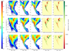 |
Fig. 1. Mϖ vs. Gaia colour GBp − GRp for the stars with G < 12 divided into three latitude ranges: first row: 30 < |b|< 90; second row: 10 < |b|< 30; third row: |b|< 10. The colour-map of the first, second, and third columns shows the logarithm of the star counts in each bin. The first column is Gaia DR2 data and the second column is the most probable model variant from Mor et al. (2018), which has an exponential SFH and whose IMF has α3 ≈ 3. The third column is for the best-fit model using a non-parametric SFH, whose IMF has α3 ≈ 2 (this work). The BGM simulations performed for this figure use the Stilism extinction map. In the fourth column we show, for each bin, the difference of star counts MP-S minus Gaia DR2 data. In the fifth column we show, for each bin, the difference of star counts G12NP-S minus Gaia DR2 data. Observational data and simulations are limited here at G < 12 and 10 < Mϖ < −1. |
The first feature of Fig. 1 that we want to comment on is the following. In the Gaia DR2 data, we can see a blob of stars (mostly in blue) below the main sequence (MS) that is not reproduced in the simulations. These are stars that are flagged with a bad colour-excess (Evans et al. 2018) in the Gaia catalogue and represent only 0.1% of our sample. By comparing the fourth and fifth columns of Fig. 1, we can see how the agreement with Gaia data is better when using the non-parametric SFH (G12NP-S). Both the excess of stars detected in the MP-S around the MS region and the deficit of stars in the region with 0.5 < (GBp − GRp)< 1.0 and 1.5 < Mϖ < 3 are clearly diminished in the new G12NP-S.
The high quality of the new information given by Gaia data reveals new discrepancies between model and data. Most of these discrepancies could come from several assumptions on the fixed ingredients of the BGM model that, as largely discussed in Sect. 7.3 of Mor et al. (2018), can impact our parameter inference. Here we discuss the discrepancies that we see in the fifth column of Fig. 1, grouped into three main areas: the red giant branch (RGB), the MS, and the region of stars with 3 < Mϖ < 4 and 0.5 < (GBp − GRp)< 1, hereafter referred to as the square region. In the RGB region, we notice that in the simulations the position of the RGB clump is shifted and that it is less extended than in the observations. In this region, the asymptotic giant branch bump is less dense in the simulations; this effect is mostly seen at intermediate latitudes. In the MS region, we detect a clear sequence where the simulation has an excess of stars and, immediately above, a clear sequence with a deficit of stars. We also notice that in the square region the simulation has a deficit of stars. This last effect is stronger at high and intermediate latitudes. As expected, these differences are caused by a mixture of factors. From a first analysis of our simulations we conclude that the thick disc modelling and the stellar evolutionary models are the two main ingredients causing the discrepancies. There are other ingredients that can contribute to these discrepancies however: the assumed colour transformation; the radial metallicity distribution; the age-metallicity relation; and the atmosphere models, which mostly have their impact in the MS and RGB; the rate of mass loss assumed in the stellar evolutionary models; the assumption of the extinction map, mostly affecting the RGB; and finally, the assumed resolution of the stellar multiple systems mostly affecting the MS. Work is in progress to more thoroughly analyse these discrepancies, to confirm their causes, and to improve the BGM model accordingly.
5. The resulting SFH and IMF
In the last column of Table 1 we show the results of the 15 inferred parameters for our fiducial case. In this section we focus on the discussion of the resulting IMF2 and the non-parametric SFH of the thin disc. In Fig. 2 we present the nine values of the local mean surface SFR as a function of age that constitute the SFH. In this figure we show the results for our fiducial case (G12NP-S). Additionally, to evaluate the impact of the choice of the extinction model in our results, we present the inferred SFH when using the Drimmel & Spergel (2001) (G12NP-D) and Marshall et al. (2006) 3 (G12NP-M) extinction maps (see Table 2). We notice that the differences in the SFR among them are not larger than 1.5σ. Regardless of the choice of the extinction map we can see a general decreasing trend from 9–10 Gyr to 6–7 Gyr ago followed by a SFR enhancement event beginning about 5 Gyr ago. This enhancement event is of about 4 Gyr in duration with a maximum at about 2–3 Gyr ago and with a final decreasing trend until the present time. We would like to point out that our results do not rule out an earlier beginning for this SFR enhancement event, nor a constant (or slightly decreasing) SFR with a value of about 7 M⊙ Gyr−1 pc−2 from 10 Gyr ago until 1 Gyr ago, with a very sharp and fast drop in the last 1 Gyr. We estimate from our best-fit model that about 50% of the mass used to generate stars throughout the life of the thin disc was expended in the period from 5 to 1 Gyr ago.
To evaluate the statistical significance of the enhancement event we compare the values of the non-parametric SFH of our fiducial case (G12NP-S) with both: (1) the values of the SFH obtained when imposing an exponential SFH in BGM and performing the fit with Gaia data (G12Exp-S results) and (2) the values of an exponential shape fitted to the G12NP-S results using the least squares method (grey dashed line in Fig. 2). This fitted exponential shape is purely mathematical and does not necessary make physical sense. The statistical significance of the points in the SFR enhancement event for the first and second cases are the following: 2.8σ and 2.5σ for the point at 2.5 Gyr ago (the relative maximum); 3σ and 1.5σ for the point at 1.5 Gyr ago, and finally 1.5σ and 0.8σ for the point at 4 Gyr ago. To evaluate the significance of the event as a whole we perform two tests with the following two null hypotheses: (1) the SFH is exponential and follows the results of the G12Exp-S variant and (2) the SFH follows the fitted mathematical exponential shape (grey dashed line in Fig. 2). In a subsequent step, for both tests, we assume that the distribution of the SFR at each age bin follows a Gaussian centred in the values given by the null hypothesis and with σ estimated from the obtained posterior PDF. Afterwards, for both null hypotheses, we compute the p-value for the points at 1.5, 2.5, and 4 Gyr ago. We finally obtain a p-value of the global event by combining the individual p-values using Fisher’s Method. The results give p-values of < 0.001 and =0.002, for hypotheses (1) and (2), respectively; we therefore reject both null hypotheses.
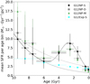 |
Fig. 2. Most probable values of the mean SFR for the age bin obtained from the posterior PDF. The vertical error bars indicate the 0.16 and 0.84 quantiles of the posterior PDF. The horizontal error bars indicate the size of the age bin. The grey and black dashed lines are, respectively, an exponential function and a distribution formed by a bounded exponential plus a Gaussian, fitted to the G12NP-S results. The grey solid line is the exponential part of this exponential plus Gaussian fit. See Table 2 for details of the SFH and extinction maps used. |
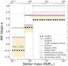 |
Fig. 3. Values of the slopes of the IMF obtained in this work together with a compilation of results in the literature. The dotted vertical lines indicate the mass limits of the three truncated power-law IMF that we adopt here (x1 = 0.5 and x2 = 1.53). See Table 2 for details on the SFH and extinction maps used. |
To mathematically characterise the SFR enhancement event we fit a bounded exponential plus a Gaussian function to the results (black dashed line in Fig. 2), obtaining for the Gaussian component μ = 2.57 Gyr and σ = 1.25 Gyr. In Fig. 2 we additionally show the exponential part of this last fit (grey solid line) where we see how the SFH of our fiducial case follows an exponential shape from 10 Gyr until 6–7 Gyr ago. From all the performed tests we conclude that the SFR enhancement that we find is statistically significant.
Our findings that the thin disc SFH does not follow a simple decreasing shape until the present are in good agreement with Snaith et al. (2015), and Haywood et al. (2016, 2018) who found, using data with metallicities and assuming a fixed IMF, the existence of an SFR quenching followed by a reactivation. Kroupa (2002a), using stellar kinematics, found the SFH to behave similarly. The relative maximum of the SFR that we find at 2–3 Gyr ago is compatible with the results of Vergely et al. (2002) and Cignoni et al. (2006) that, using HIPPARCOS data in a sphere of 80 pc around the Sun and assuming a fixed IMF, found maximum peaks at 1.75–2 Gyr ago and 2–3 Gyr ago, respectively. Recently, Bernard (2018), in a tentative work using TGAS data, pointed towards the existence of a relative maximum also located 2–3 Gyr ago.
In Fig. 3 we show the resulting slopes (α) of the inferred IMF as a function of stellar mass and a compilation of results in the literature. For the mass range between 0.5 M⊙ and 1.53 M⊙ we find α2 = 1.3 ± 0.3, in very good agreement with Rybizki & Just (2015) who found α = 1.49 ± 0.08 (in the range 0.5 M⊙ < M < 1.4 M⊙). For masses larger than 1.53 M⊙ we find  , which is flatter than the α3 obtained by Salpeter (1955) and Kroupa (2002b). For the low-mass range (0.09 M⊙ < M < 0.5 M⊙) we obtain values between α1 = −1 and α1 = 0.5. We must keep in mind our estimation that about 99.6% of the stars in our sample have masses between 0.5 M⊙ and 10 M⊙, with only 0.1% of the stars in our sample belonging to the lowest mass range, and that of the order of 104 stars have M > 10 M⊙. We also want to compare our results with two works that consider a non-universal IMF. These are the recent works of Dib & Basu (2018) and Jeřábková et al. (2018; see Appendix A). We note that, as in our results, their IMFs have a shallower shape than the values of Kroupa or Salpeter. The information from Gaia parallaxes, when imposing an exponential SFH, brings the resulting α3 to be ≈2.5. This is flatter than in our previous works (Mor et al. 2017, 2018) but compatible with the α3 ≈ 2.7 of the IGIMF (e.g. Kroupa et al. 2013). When we adopt a non-parametric SFH we find α3 ≈ 2, more in the direction of Zonoozi et al. (2019). We know from Mor et al. (2018; e.g. their Fig. 7) that when characterising the IGIMF from star counts the correlation of α3 with the SFH is high. In our previous works, the fact that we were imposing an exponential SFH resulted in a steeper α3. These correlations between the α3 and the SFH are also observed in our present work. We find that the α3 is anti-correlated with the four
  values for the age bins from 0.1 to 5 Gyr, with a Pearson’s correlation coefficient going from about −0.8 to about −0.5. We also note that these four surface densities (
 ) are also correlated among them, with coefficients from about 0.3 to 0.5. We want to emphasise that the effects of these correlations in the results (Table 1, Figs. 2 and 3) are already taken into account when we provide the 0.16 and 0.84 quantiles of the posterior PDFs. From the surface SFR of the youngest population (
 Gyr−1 pc−2) we find the present SFR in the disc to be about 1 M⊙/yr. This result is very sensitive to the disc scaling of the youngest population. We also find a radial scale length of
 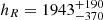 compatible with Robin et al. (2012). For robustness we repeated our analysis by adding to the Gaia DR2 parallaxes the offset of 0.029 mas reported in Lindegren et al. (2018), concluding that the impact on the derived IMF and SFH is much smaller than the impact of the choice of the extinction map.
6. Conclusion
For the first time we have considered a non-parametric SFH for the thin disc in the BGM model. This new step, together with the capability of the Gaia DR2 parallaxes to break degeneracies between different stellar populations, allowed us to better constrain the thin disc SFH and IMF. The resulting SFH shows a decreasing trend from 9–10 to 6–7 Gyr ago that is consistent with the quenching observed in a cosmological context for redshifts z < 1.8 (e.g. Rowan-Robinson et al. 2016) and is also compatible with the evidence of the quenching in the Milky Way reported in Haywood et al. (2018). The quenching that we find could be linked to a previous merger event. Simulations in the framework of ΛCDM show that after a merger, there is an enhancement of the star formation followed by a quenching (e.g. Di Matteo et al. 2008, Fig. 4). This would be compatible with the thick-disc formation scenario recently proposed in Helmi et al. (2018) with a merger which occurred more than 10 Gyr ago. As suggested in other works, the quenching that we find could also be partially produced by the presence of a galactic bar (Haywood et al. 2016; Khoperskov et al. 2018). The two quenching mechanisms discussed here are not mutually exclusive but complementary. After the quenching, we detect a 4 Gyr duration SFR-enhancement event starting at about 5 Gyr ago and with a maximum at 2–3 Gyr ago. The large timescale of this recent SFR enhancement event, together with the large amount of mass that we estimate to be involved in it (see Sect. 5), lead us to propose that this recent event is not intrinsic to the disc but is produced by an external perturbation. Furthermore, the slow increase of the star formation process, its duration, as well as the high absolute value of the maximum suggest that this could be produced by a recent merger with a gas-rich satellite galaxy that could have started between about 5 and 7 Gyr ago. However, an analysis of other stellar parameters (e.g. metallicities) would be needed to favour this hypothesis over other possible scenarios.
Work is in progress to more thoroughly analyse the Gaia DR2 data by extending our study to fainter magnitudes, updating the stellar evolutionary models and the thick disc modelling.
We know from Kendall & Stuart (1973) and Bienaymé et al. (1987) that the Poissonian distance is a good choice for the comparison. For simplicity it can be understood as a goodness-of-fit: the shorter the Poissonian distance, the closer the simulation to the observations.
As largely discussed in Mor et al. (2017), the IMF considered in BGM is a composite IMF (or Integrated Galactic IMF; IGIMF).
The Marshall et al. (2006) extinction map covers the longitude ranges −100 < l < 100 and the latitude ranges |b|< 10. Therefore, Drimmel map is used for the rest of the sky.
Acknowledgments
We thank the anonymous referee for the constructive report which helped to improve the quality of the work. Special thanks are to N. Lagarde, C. Charbonnel, and C. Reylé for very useful discussions. This work was supported by the MINECO (Spanish Ministry of Economy) – FEDER through grant ESP2016-80079-C2-1-R and MDM-2014-0369 of ICCUB (Unidad de Excelencia “María de Maeztu”), the French Agence Nationale de la Recherche under contract ANR-2010-BLAN-0508-01OTP and the European Community’s Seventh Framework Programme (FP7/2007-2013) under grant agreement GENIUS FP7 – 606740. We also acknowledge the team of engineers (GaiaUB-ICCUB) in charge to set up the Big Data platform (GDAF) at University of Barcelona. We also acknowledge the International Space Science Institute, Bern, Switzerland for providing financial support and meeting facilities. This work has made use of data from the European Space Agency (ESA) mission Gaia (https://www.cosmos.esa.int/gaia), processed by the Gaia Data Processing and Analysis Consortium (DPAC, https://www.cosmos.esa.int/web/gaia/dpac/consortium). Funding for the DPAC has been provided by national institutions, in particular the institutions participating in the Gaia Multilateral Agreement.
References
- Antoja, T., Helmi, A., Romero-Gómez, M., et al. 2018, Nature, 561, 360 [NASA ADS] [CrossRef] [Google Scholar]
- Aumer, M., & Binney, J. J. 2009, MNRAS, 397, 1286 [NASA ADS] [CrossRef] [Google Scholar]
- Bernard, E. J. 2018, in Rediscovering Our Galaxy, eds. C. Chiappini, I. Minchev, E. Starkenburg, & M. Valentini, IAU Symp., 334, 158 [NASA ADS] [Google Scholar]
- Bienaymé, O., Robin, A. C., & Creze, M. 1987, A&A, 180, 94 [Google Scholar]
- Cignoni, M., Degl’Innocenti, S., Prada Moroni, P. G., & Shore, S. N. 2006, A&A, 459, 783 [Google Scholar]
- Czekaj, M. A., Robin, A. C., Figueras, F., Luri, X., & Haywood, M. 2014, A&A, 564, A102 [NASA ADS] [CrossRef] [EDP Sciences] [Google Scholar]
- Dib, S., & Basu, S. 2018, A&A, 614, A43 [NASA ADS] [CrossRef] [EDP Sciences] [Google Scholar]
- Di Matteo, P., Bournaud, F., Martig, M., et al. 2008, A&A, 492, 31 [NASA ADS] [CrossRef] [EDP Sciences] [Google Scholar]
- Drimmel, R., & Spergel, D. N. 2001, ApJ, 556, 181 [NASA ADS] [CrossRef] [Google Scholar]
- Evans, D. W., Riello, M., De Angeli, F., et al. 2018, A&A, 616, A4 [NASA ADS] [CrossRef] [EDP Sciences] [Google Scholar]
- Gaia Collaboration (Prusti, T., et al.) 2016, A&A, 595, A1 [NASA ADS] [CrossRef] [EDP Sciences] [Google Scholar]
- Gaia Collaboration (Brown, A. G. A., et al.) 2018, A&A, 616, A1 [NASA ADS] [CrossRef] [EDP Sciences] [Google Scholar]
- Gilmore, G. 2001, in Galaxy Disks and Disk Galaxies, eds. J. G. Funes, & E. M. Corsini, ASP Conf. Ser., 230, 3 [NASA ADS] [Google Scholar]
- Haywood, M., Robin, A. C., & Creze, M. 1997, A&A, 320, 428 [NASA ADS] [Google Scholar]
- Haywood, M., Lehnert, M. D., Di Matteo, P., et al. 2016, A&A, 589, A66 [NASA ADS] [CrossRef] [EDP Sciences] [PubMed] [Google Scholar]
- Haywood, M., Di Matteo, P., Lehnert, M., et al. 2018, A&A, 618, A78 [NASA ADS] [CrossRef] [EDP Sciences] [Google Scholar]
- Helmi, A., Babusiaux, C., Koppelman, H. H., et al. 2018, Nature, 563, 85 [NASA ADS] [CrossRef] [Google Scholar]
- Høg, E., Fabricius, C., Makarov, V. V., et al. 2000, A&A, 355, L27 [Google Scholar]
- Jennings, E., & Madigan, M. 2017, Astron. Comput., 19, 16 [NASA ADS] [CrossRef] [Google Scholar]
- Jeřábková, T., Hasani Zonoozi, A., Kroupa, P., et al. 2018, A&A, 620, A39 [NASA ADS] [CrossRef] [EDP Sciences] [Google Scholar]
- Kendall, M. G., & Stuart, A. 1973, The Advanced Theory of Statistics, Vol. 2, Ch. 18. (London: Griffin) [Google Scholar]
- Khoperskov, S., Haywood, M., Di Matteo, P., Lehnert, M. D., & Combes, F. 2018, A&A, 609, A60 [NASA ADS] [CrossRef] [EDP Sciences] [Google Scholar]
- Kroupa, P. 2002a, MNRAS, 330, 707 [NASA ADS] [CrossRef] [Google Scholar]
- Kroupa, P. 2002b, Science, 295, 82 [NASA ADS] [CrossRef] [PubMed] [Google Scholar]
- Kroupa, P., Weidner, C., Pflamm-Altenburg, J., et al. 2013, in The Stellar and Sub-Stellar Initial Mass Function of Simple and Composite Populations, eds. T. D. Oswalt, & G. Gilmore, 115 [Google Scholar]
- Kruijssen, J. M. D., Pfeffer, J. L., Reina-Campos, M., Crain, R. A., & Bastian, N. 2019, MNRAS, in press [arXiv:1806.05680] [Google Scholar]
- Lallement, R., Capitanio, L., Ruiz-Dern, L., et al. 2018, A&A, 616, A132 [NASA ADS] [CrossRef] [EDP Sciences] [Google Scholar]
- Lindegren, L., Hernández, J., Bombrun, A., et al. 2018, A&A, 616, A2 [NASA ADS] [CrossRef] [EDP Sciences] [Google Scholar]
- Marshall, D. J., Robin, A. C., Reylé, C., Schultheis, M., & Picaud, S. 2006, A&A, 453, 635 [NASA ADS] [CrossRef] [EDP Sciences] [Google Scholar]
- Mor, R., Robin, A. C., Figueras, F., & Lemasle, B. 2017, A&A, 599, A17 [NASA ADS] [CrossRef] [EDP Sciences] [Google Scholar]
- Mor, R., Robin, A. C., Figueras, F., & Antoja, T. 2018, A&A, 620, A79 [Google Scholar]
- Robin, A. C., Reylé, C., Derrière, S., & Picaud, S. 2003, A&A, 409, 523 [NASA ADS] [CrossRef] [EDP Sciences] [Google Scholar]
- Robin, A. C., Marshall, D. J., Schultheis, M., & Reylé, C. 2012, A&A, 538, A106 [NASA ADS] [CrossRef] [EDP Sciences] [Google Scholar]
- Robin, A. C., Reylé, C., Fliri, J., et al. 2014, A&A, 569, A13 [NASA ADS] [CrossRef] [EDP Sciences] [Google Scholar]
- Rowan-Robinson, M., Oliver, S., Wang, L., et al. 2016, MNRAS, 461, 1100 [NASA ADS] [CrossRef] [Google Scholar]
- Rybizki, J., & Just, A. 2015, MNRAS, 447, 3880 [NASA ADS] [CrossRef] [Google Scholar]
- Salpeter, E. E. 1955, ApJ, 121, 161 [Google Scholar]
- Snaith, O., Haywood, M., Di Matteo, P., et al. 2015, A&A, 578, A87 [NASA ADS] [CrossRef] [EDP Sciences] [Google Scholar]
- Stewart, K. R., Bullock, J. S., Wechsler, R. H., Maller, A. H., & Zentner, A. R. 2008, ApJ, 683, 597 [NASA ADS] [CrossRef] [Google Scholar]
- Vergely, J. L., Lançon, A., & Mouhcine, M. 2002, A&A, 394, 807 [NASA ADS] [CrossRef] [EDP Sciences] [Google Scholar]
- Yan, Z., Jerabkova, T., & Kroupa, P. 2017, A&A, 607, A126 [NASA ADS] [CrossRef] [EDP Sciences] [Google Scholar]
- Zonoozi, A. H., Mahani, H., & Kroupa, P. 2019, MNRAS, 483, 46 [NASA ADS] [CrossRef] [Google Scholar]
Appendix A: Treatment of the IMFs from Dib & Basu (2018) and Jeřábková et al. (2018)
To be able to compare the IMFs of Dib & Basu (2018) and Jeřábková et al. (2018) with the IMF that we obtain in this work we need to perform an adequate treatment. For the case of Dib & Basu (2018), to be able to compare the slopes, we fit a three truncated power-law IMF to their results when they assume aΓ = 0.5, aγ = 0.5, and aMch = 0.5 (see their Fig. 1). We plot this result in Fig. 3. The case of Jeřábková et al. (2018) is slightly more complex as their IMF depends on the SFR and metallicity. From our results we estimate a mean SFR (in M⊙/yr) and a mean metallicity for each one of the age bins considered. Then from Yan et al. (2017) and Jeřábková et al. (2018) we get a resulting IMF for each age bin (using galIMF4). Finally we compute a weighted mean of the IMF depending on the total mass for each age bin. The total integrated galactic IMF is then plotted in Fig. 3.
All Tables
Summary of the considered model variants, the adopted SFH, extinction map, data used for the fitting and Poissonian distance (δP).
All Figures
|
Fig. 1. Mϖ vs. Gaia colour GBp − GRp for the stars with G < 12 divided into three latitude ranges: first row: 30 < |b|< 90; second row: 10 < |b|< 30; third row: |b|< 10. The colour-map of the first, second, and third columns shows the logarithm of the star counts in each bin. The first column is Gaia DR2 data and the second column is the most probable model variant from Mor et al. (2018), which has an exponential SFH and whose IMF has α3 ≈ 3. The third column is for the best-fit model using a non-parametric SFH, whose IMF has α3 ≈ 2 (this work). The BGM simulations performed for this figure use the Stilism extinction map. In the fourth column we show, for each bin, the difference of star counts MP-S minus Gaia DR2 data. In the fifth column we show, for each bin, the difference of star counts G12NP-S minus Gaia DR2 data. Observational data and simulations are limited here at G < 12 and 10 < Mϖ < −1. |
| In the text | |
|
Fig. 2. Most probable values of the mean SFR for the age bin obtained from the posterior PDF. The vertical error bars indicate the 0.16 and 0.84 quantiles of the posterior PDF. The horizontal error bars indicate the size of the age bin. The grey and black dashed lines are, respectively, an exponential function and a distribution formed by a bounded exponential plus a Gaussian, fitted to the G12NP-S results. The grey solid line is the exponential part of this exponential plus Gaussian fit. See Table 2 for details of the SFH and extinction maps used. |
| In the text | |
|
Fig. 3. Values of the slopes of the IMF obtained in this work together with a compilation of results in the literature. The dotted vertical lines indicate the mass limits of the three truncated power-law IMF that we adopt here (x1 = 0.5 and x2 = 1.53). See Table 2 for details on the SFH and extinction maps used. |
| In the text | |
Current usage metrics show cumulative count of Article Views (full-text article views including HTML views, PDF and ePub downloads, according to the available data) and Abstracts Views on Vision4Press platform.
Data correspond to usage on the plateform after 2015. The current usage metrics is available 48-96 hours after online publication and is updated daily on week days.
Initial download of the metrics may take a while.