| Issue |
A&A
Volume 621, January 2019
|
|
|---|---|---|
| Article Number | A121 | |
| Number of page(s) | 8 | |
| Section | Interstellar and circumstellar matter | |
| DOI | https://doi.org/10.1051/0004-6361/201834346 | |
| Published online | 16 January 2019 | |
Detection of nitrogen gas in the β Pictoris circumstellar disc
1
Department of Physics, University of Warwick,
Coventry CV4 7AL,
UK
e-mail: This email address is being protected from spambots. You need JavaScript enabled to view it.
2
Centre for Exoplanets and Habitability, University of Warwick,
Coventry CV4 7AL,
UK
3
Leiden Observatory, Leiden University,
Postbus 9513,
2300
RA Leiden,
The Netherlands
4
CNRS, UMR 7095, Institut d’Astrophysique de Paris,
75014
Paris,
France
5
Institut d’Astrophysique de Paris,
75014
Paris,
France
6
University of British Columbia,
2329 West Mall,
Vancouver,
BC,
V6T 1Z4,
Canada
7
Observatoire de l’Université de Genève,
51 chemin des Maillettes,
1290
Sauverny,
Switzerland
Received:
29
September
2018
Accepted:
9
November
2018
Abstract
Context. The gas composition of the debris disc surrounding β Pictoris is rich in carbon and oxygen relative to solar abundances. Two possible scenarios have been proposed to explain this enrichment. The preferential production scenario suggests that the produced gas may be naturally rich in carbon and oxygen, while the alternative preferential depletion scenario states that the enrichment has evolved to the current state from a gas with solar-like abundances. In the latter case, the radiation pressure from the star expels the gas outwards, leaving behind species that are less sensitive to stellar radiation such as C and O. Nitrogen is not sensitive to radiation pressure either as a result of its low oscillator strength, which would make it also overabundant under the preferential depletion scenario. The abundance of nitrogen in the disc may therefore provide clues to why C and O are overabundant.
Aims. We aim to measure the nitrogen column density in the direction of β Pictoris (including contributions by the interstellar medium and circumstellar disc), and use this information to distinguish these different scenarios to explain the C and O overabundance.
Methods. Using far-UV spectroscopic data collected by the Hubble Space Telescope’s Cosmic Origins Spectrograph (COS) instrument, we analysed the spectrum and characterised the NI triplet by modelling the absorption lines.
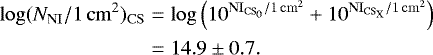
Results. We measure the nitrogen column density in the direction of β Pictoris for the first time, and find it to be log(NNI/1 cm2) = 14.9 ± 0.7. The nitrogen gas is found to be consistent with solar abundances and Halley dust. We also measure an upper limit for the column density of MnII in the disc at log(NMnII/1 cm2)CS = 12.7+0.1 and calculate the column density of SIII** in the disc to be log(NSIII★★/1 cm2)CSX = 14.2 ± 0.1. Both results are in good agreement with previous studies.
Conclusions. The solar nitrogen abundance supports the preferential production hypothesis, in which the composition of gas in β Pictoris is the result of photodesorption from icy grains that are rich in C and O or collisional vaporisation of C- and O-rich dust in the disc. It does not support the hypothesis that C and O are overabundant because C and O are insensitive to radiation pressure, which would cause them to accumulate in the disc.
Key words: stars: early-type / stars: individual: β Pictoris / circumstellar matter
© ESO 2019
1 Introduction
β Pictoris (β Pic) is a young 23 ± 3 Myr (Mamajek & Bell 2014) planetary system that hosts a nearly edge-on debris disc that is composed of dust and gas. The gas in the disc is not thought to be primordial, but rather continually replenished through evaporation and collisions between dust grains. The detection of the CO molecule (Vidal-Madjar et al. 1994; Dent et al. 2014; Matrà et al. 2017) is evidence that new gas is being produced because the typical lifetime of the CO molecule is very short, ~120 yr (Visser et al. 2009). The presence of UV photons from the ambient interstellar medium rapidly dissociates CO into C and O, which then evolves by viscous spreading (Kral et al. 2016, 2017).
Observations have shown that the circumstellar (CS) disc has a particularly large overabundance of C and O relative to a solar abundance (Roberge et al. 2006; Brandeker 2011). Xie et al. (2013) introduced two opposing hypotheses to explain the origin of this overabundance. The first hypothesis, which they named preferential production, holds when the gas is produced with an enriched C and O abundance. Such an enrichment could be created through processes that release gas from solid bodies with an inherently high C and O abundance, such as bodies rich in CO (Kral et al. 2016). The main gas-producing processes are photodesorption off the grains, a non-thermal desorption mechanism that releases gas by UV-flux (Grigorieva et al. 2007), collisional vaporisation of the dust in the disc (Czechowski & Mann 2007), cometary collisions (Zuckerman & Song 2012), and sublimating exocomets (Ferlet et al. 1987; Beust et al. 1990; Lecavelier Des Etangs et al. 1996). Preferential depletion, the second of the two hypotheses by Xie et al. (2013), suggests that the gas evolves to have an elevated C and O abundance from an originally solar abundance (≳ 1 dex). Metallic elements subject to strong radiation forces, such as Na and Fe, could deplete more quickly than C and O, for which the radiation force is negligible, which would lead to an overabundance of C and O. The presence of the overabundant C and O has been invoked as an explanation for why other gas species seen in the CS disc have not been blown away by the radiation pressure of the star and why the orbital motion of the gas is consistent with Keplerian rotation (Fernández et al. 2006).
A column density measurement of nitrogen could help distinguish between these two hypotheses to explain the overabundance of C and O. If the N/Fe column density were found to be similar to the N/Fe solar abundance, this would speak in favour of preferential production. If the column density of N were found to be high, this would support the preferential depletion hypothesis. The reason is that N, like C and O, is not sensitive to radiation forces and thus should be overabundant compared to radiation-sensitive species under the preferential depletion scenario.
A column density measurement of N might also shed light on the gas production mechanism in the β Pic CS disc. Molecular abundance analyses of comets in the solar system indicate that cometary coma consist mostly of H2 O (~ 90%) followed by CO (~5%) and CO2 ~ 3% and that nitrogen-bearing molecules such as N2, NH3, and CN are only minor constituents (e.g. Krankowsky et al. 1986; Eberhardt et al. 1987; Wyckoff et al. 1991). Although previous studies have measured the cometary coma and not the internal abundances, it is unlikely that comets produce significant amounts of N.
In this paper, we present the first detection of nitrogen in the β Pic disc based upon observations obtained using the Hubble Space Telescope (HST) together with the far-UV Cosmic Origins Spectrograph (COS) instrument. In Sect. 2, we present the observational setup and technique used. The analysis of the data, which includes airglow removal, spectral alignment, and the combination and modelling of the NI lines, is presented in Sect. 3. The results are presented in Sect. 4 with a discussion of the obtained NI abundance measurements in Sect. 5. The main findings are summarised in Sect. 6, where we also highlight the significance of the NI abundance measurement.
2 Observations
The far-UV observations of β Pic were obtained with the COS on the HST using the TIME-TAG mode and the G130M grating. The observations were made using the primary science aperture, which has a field stop of 2.5′′ in diameter. The observations consisted of a total of 11 visits and 31 orbits, conducted between February 2014 and May 2018. The central wavelength was first set at 1291 Å, but upon inspection of the data, a decision was made to change the central wavelength setting to 1327 Å for all observations after 2016 to avoid the photon-poor region towards the shortest wavelengths. The two central wavelength positions overlap in the 1171–1279 Å and 1327–1433 Å wavelength regions.
To avoid contamination by geocoronal emission (airglow), we used the airglow virtual motion (AVM) technique, where the target is deliberately offset along the dispersion axis, thereby separating the target spectrum from the stationary airglow spectrum. A more detailed description of this method can be found in the appendix of Wilson et al. (2017). The data were all reduced using the COSTOOLS pipeline (Fox et al. 2015) version 3.2.1 (2017-04-28).
3 Analysis
3.1 Airglow modelling and subtraction
The HST is located in Earth’s tenuous atmosphere (in the exosphere) where H, N, and O are present in sufficient quantities to be detected in emission at far-UV wavelengths. These emission lines, known as airglow, are present in the data, and can, if left un-corrected, reduce the accuracy of the column density estimates. We removed theairglow contamination by subtracting an airglow template made from combining several airglow-only observations. The airglow templates were created using data obtained during our previous observations (Wilson et al. 2017)in combination with airglow templates made available on the Space Telescope Science Institute (STScI) website1.
The final airglow-subtracted data, F, were created by subtracting the airglow template, FAG, scaled by a factor, C, from the original contaminated data spectrum, Ftot. This is expressed in the following equation:
 (1)
(1)
A detailed explanation of these latter steps, including the methods for calculating C, are explained in the Appendices A.1–A.3.
3.2 Choice of line spread function
Mid-frequency errors caused by polishing irregularities in the HST primary and secondary mirrors cause the spectroscopic line-spread function (LSF) to exhibit extended wings with a core that is broader and shallower when compared to a Gaussian LSF. For our modelling, we chose to use the tabulated LSF (LP3) available on the STScI website2. Since the shape of the LSF changes with wavelength, we chose the tabulated LSF closest to our wavelength region of interest: G130M/1222. The shape of the LSF reduces our ability to detect faint and narrow spectral features. It is therefore likely that we are not particularly sensitive to the fainter MnII and SIII** that exist close to the NI lines. Furthermore, the non-Gaussian line wings also make it hard to detect closely spaced narrow spectral features. This limits the complexity of our model to only a few absorption components.
3.3 Modelling the NI lines
The NI absorption lines in the β Pic spectrum were modelled using Voigt profiles. We computed the Voigt profile (a convolution of a Gaussian and a Lorentzian profile) as the real part of the Faddeeva function, computed with standard Python libraries (scipy.special.wofz). Each nitrogen line in the main triplet (1199.5496, 1200.2233, and 1200.7098 Å) was modelled and fitted simultaneously over a predefined spectral region (1198.48–1202.35 Å). The additional NI triplet at (1134.1653, 1134.4149 and 1134.9803 Å) towards the end of the detector and the weak lines at 1159.8168 and 1160.9366 Å have weak line strengths that result in line depths that lie below the local noise level, so they were not included in the fitting. When we found a satisfactory model for the main NI triplet at ~ 1200Å, we compared this solution with the other weaker NI line regions and found that our model is consistent with these much weaker lines. We also modelled the MnII and SIII** lines at 1199.39, 1201.12 Å and 1200.97 Å, respectively, as they partially overlap with the NI lines. The separate SIII** line at 1201.73 Å was used to break any degeneracy between the NI line at 1200.71 Å and the SIII** line at 1200.97 Å.
3.3.1 Choosing the number of model components
We initially fitted the absorption lines using a two-component model consisting of one component that represented the interstellar medium (ISM) and another that represented the circumstellar gas disc. The resulting fit was poor, suggesting the presence of a third component. This third component was added and called CSX, and when we included it, the value of the χ2 decreased from 1.6 (with 10 free parameters) to 1.0 (with 15 free parameters). This decreased the Bayesian information criterion (Schwarz et al. 1978) from 646 to 451 and the Akaike information criterion (Akaike 1974) from 607 to 409. Adding a fourth component did not improve the fit, however, so we settled on this three-component model. The CSX component, which was left free to vary in radial velocity space, gave the best fit close to the rest frame of β Pic at 20.0 km s−1 (Brandeker et al. 2004; Gontcharov 2006). The continuum was modelled using a second-order polynomial.
3.3.2 Selecting the free component parameters
In the absence of reliable lines for which to check the wavelength calibration locally, we took the liberty of not constraining the ISM (vISM) and CS0 ( ) bulk velocities to their literature values. However, since the ISM component has been well-constrained in previous studies to be offset by −10 km s−1 relative to the stellar radial velocity component (Vidal-Madjar et al. 1994; Lallement et al. 1995), we set this requirement and allowed the two parameters to vary together, provided that
  km s−1 was maintained. Except for this radial velocity constraint, the only ISM-related parameter left free to vary was the nitrogen column density:
  . The fixed ISM parameters were TISM = 7000 K (the temperature of the ISM) and ξISM = 1.5 km s−1 (the turbulent broadening of the ISM). These two values follow from studies of the interstellar medium towards β Pic and other nearby stars, such as Bertin et al. (1995) and Lallement et al. (1995).
For both circumstellar components, the column density and turbulent broadening (ξ) were set as free parameters. The bulk velocity of the CSX component was also allowed to vary freely. The temperature of the CS gas is unknown. However, to avoid the degeneracy introduced when the turbulent velocity and the temperature are modelled simultaneously, we fixed the CS gas temperature to 10 K for the two CS components. The relationship between the parameters is expressed mathematically as
 (2)
(2)
where b is the width of the lines, T is the temperature, k is the Boltzmann constant, m is the mass of the considered species, and ξ is the turbulent broadening (also sometimes referred to as microturbulent velocity).
3.4 Fit to the data
We fitted the NI triplet in conjunction with the MnII and SIII** lines, with MnII overlapping the blue side of bluest NI line. We did not model SIII** in the ISM component as sulphur will instead exist in the form of SII. We checked and found that only a model with a low SIII** column density provides a fit that is consistent with the data.
We employed a least-squares optimisation to the data using the scipy.optimize.leastsq package (Jones et al. 2001) to obtain initial starting parameters for a Markov chain Monte Carlo (MCMC) run using the emcee code described in Foreman-Mackey et al. (2013). We ran 200 MCMC walkers with a total of 10 100 steps each, with 100 burn-in steps. This resulted in a total of two million steps, of which ~25% were accepted. The posterior probability distributions for the free model parameters were calculated using the corner plot code of Foreman-Mackey (2016) where the marginalised 1D distributions were used to calculate the mean values and the uncertainties on each free parameter (see Table 1).
Mean and median values and uncertainties of the posterior probability distributions generated with the MCMC method.
4 Results
4.1 Saturated NI lines
The results from the best fit (and MCMC) show that the CS0 component is completely saturated (shown by the cyan lines, which reach a flux of 0 in Fig. 1). The ISM component is partially saturated. The saturation leads to larger uncertainties on  that reach a magnitude uncertainty of 0.7 because an increase in column density does not deepen the absorption signature, but instead widens the absorption profile, which is then partially absorbed by the CSX component. This is shown by the broad posterior distribution of
  values in Fig. 3. Interestingly, although the CSX is free to vary in radial velocity, it has the same radial velocity as the CS0 component (within 1σ). The same bulk velocity values indicate that the CS0 and CSX might describe the same gas. This is discussed in more detail in Sect. 5.
We find a system velocity for β Pic of  km s−1, which is consistent with the accepted value of ~ 20.5 km s−1 (Hobbs et al. 1985; Brandeker et al. 2004). The slight difference between the values is likely caused by uncertainties in the wavelength solution.
To estimate the total column density of circumstellar NI gas, we added the two circumstellar components together:
 (3)
(3)
We compared the ratio of the N/Fe column density (normalised to Si) with solar abundances, CI chondrites, and Halley dust in Fig. 2. It shows that the NI abundance is consistent with solar and Halley dust abundances, but is inconsistent with CI chondrites.
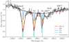 |
Fig. 1 Measured flux as a function of wavelength (HST rest frame) for the NI lines at ~ 1200Å. The black spectrum represents the combined data, and the thicker parts indicate the region we used to fit the continuum, which is shown as a black solid line. The coloured lines show the individual components. The cyan line shows the individual absorption profiles before they were convolved by the instrumental LSF. |
4.2 Indirect estimate of the H column density of the ISM in the direction of β Pic
Using the HST and the Goddard High Resolution Spectrograph (GHRS), Meyer et al. (1997) conducted observationsof the interstellar NI and found a value for the mean interstellar gas-phase N/H abundance at (7.5 ± 0.4) × 10−5. Furthermore, they reported no statistically significant variations in the measured N abundances from sight line to sight line and no evidence of density-dependent nitrogen depletion from the gas phase. We estimated the total hydrogen column density in the ISM given the value for the NI ISM column density calculated in this paper and assuming N(NI) ≈ N(Ntotal). Based on the NI ISM column density, we calculate that the HI ISM value in the direction of β Pic is  . This is consistent with Wilson et al. (2017), where this value was found to be 18.2± 0.1.
4.3 Column density estimates for MnII and SIII**
We are ableto place robust upper limits on the column density estimates for MnII and SIII**. The lower limit is generally unobtainable as the absorption signature is so small that it becomes indistinguishable from the noise. The MnII posterior distributions are not flat topped, however, which one would expect when the absorbing component becomes indistinguishable from the noise. As there seems to be a preferred column density value, we estimated the MnII column density by calculating the mode of the MnII column density distributions and found them to be 12.2+0.1 and 12.6+0.1 for the CS0 and CSX components, respectively. Added together, we obtain a value of  or (5.0 ± 1.2) × 1012 atoms cm−2. This value is consistent with the value of 3.8 × 10¹² atoms cm−2 reported by Lagrange et al. (1998).
The total SIII** CS column density is dominated by the CSX component, which is  or (1.6 ± 0.7) × 1014 atoms cm−2. Lagrange et al. (1998) measured a value of 1.1 × 10¹⁴ atoms cm−2, which is also consistent with our measurement.
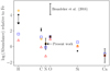 |
Fig. 2 Abundances of the β Pic gas disc (black circles) compared to solar abundances (orange Sun symbols), CI chondrites (red triangles) and Halley dust (blue squares). The abundances are given relative to iron (Fe), and the figure is adapted from Fig. 2 of Roberge et al. (2006). The OI detection by Brandeker et al. (2016), who used the Herschel telescope, represents a range of possible values that depend on the spatial distribution of the O gas in the CS disc. The OI column density estimate by Roberge et al. (2006; represented by the black circle) could represent a lower column density limit because of the challenges associated with measuring optically thick OI lines (see Brandeker 2011 and Fig. S1 in Roberge et al. 2006). The CI chondrites consistently show low abundances for the volatile elements H, C, N, and O, which is expected as they were in a gaseous state when the meteorite formed and therefore did not condense or accrete. |
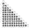 |
Fig. 3 Corner plot showing the 1D and 2D projections of the posterior probability distributions for the free parameters. The blue dashed lines indicate the mean of the distribution. The black dashed lines in each of the 1D histograms represent the 1 σ deviations (68% of the mass). The central dashed line indicates the median value. The solid black lines in each of the 2D histograms represent the 1, 2, and 3 σ levels, respectively (with 1 σ = 39.3% of the volume). The red dashed lines indicate the mode of the distribution. The uncertainty for the parameters that only have an upper uncertainty was calculated assuming a truncated Gaussian distribution. |
5 Discussion
5.1 Implications of a solar NI abundance
The column density of NI relative to iron is shown in Fig. 2. The NI column density is consistent with solar abundances, unlike C and O, which are overabundant.
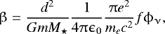
The preferential depletion scenario presented in Xie et al. (2013) suggests that the overabundance of C and O is due to their accumulation in the disc. As the radiation from β Pic depletes the metallic elements (susceptible to radiation pressure), such as Na, Mg, Ca, and Fe, the radiation-resilient species remain in the gas disc, resulting in an C and O overabundance. Under such a scenario, we would expect N to be overabundant as well, as N has a low sensitivity to radiation pressure, like C and O. This can be demonstrated by evaluating the ratio of the radiation pressure to stellar gravity, which is expressed as β:
 (4)
(4)
where d is the distance to the star, G is the gravitational constant, m is the mass of the ion under consideration, M⋆ is the stellar mass, ϵ0 the permittivity of free space, e the elementary charge, me the mass of the electron, c the speed of light, f the oscillator strength of the transition, and ϕν is the stellar flux at the considered wavelength (per unit frequency). We calculated this quantity using the following values: f =0.130 (for the strongest line), m = 14 u, λ = 1199.55Å, stellar flux = 1.0 × 10⁻¹⁴ erg s−1 cm−2 Å−1, d = 19.3 pc, and M⋆ = 1.75 M⊙. This returns β ≃ 3.6 × 10⁻⁴. While determining the exact influence of radiation pressure on nitrogen atoms would require a dynamical model, such a low value for β indicates that it should have a negligible effect. Despite these very weak effects from radiation pressure, we do not find an overabundance of nitrogen in the β Pictoris disc. Other papers have also shown no clear deficiency in radiation-sensitive species such as Na and Ca (Lagrange et al. 1998), which also seems to disfavour the preferential depletion scenario.
The preferential production scenario, also proposed by Xie et al. (2013), suggests that the overabundance is the result of gas being produced from materials rich in C and O. This includes photodesorption from C and O-rich icy grains (Grigorieva et al. 2007) and collisional vaporisation of the dust in the disc (Czechowski & Mann 2007). Unlike preferential depletion, this scenario does not infer high N abundances and is thus more compatible with the near-solar NI abundance measured here.
5.2 Origin and dynamics of the NI gas
The absorption components that we used to model the shape of the NI absorption lines may provide us with hints at both the origin and dynamics of the NI gas. The two absorbing circumstellar components, CS0 and CSX, were not constrained to particular radial velocity values, but provided the best fit when their radial velocities matched that of the star. This indicates an absence of detectable amounts of NI falling in towards the star. The clearly asymmetric HI Ly-α line presented in Wilson et al. (2017), on the other hand, indicates that HI gas is falling in towards the star. The HI gas is thought to be originating from the dissociation of water molecules from evaporating exocomets. The fact that we do not see similar asymmetric line profiles in NI is perhaps not surprising. In solar system comets, nitrogen-bearing molecules are only minor constituents (Eberhardt et al. 1987), which means that if β Pic comets are similar, we would not expect the NI lines to be asymmetric. This does not exclude the possibility that NI might originate from exocomets, however, as we argue in Sect. 5.3.
5.3 Role of exocomets
The NI column density measurements are dominated by the narrow absorption feature, CS0, which has a line width of  km s−1. With a similar line width observed in FeI (Vidal-Madjar et al. 2017), this absorption feature likely traces a stable band of circumstellar material that orbits β Pic. The origin of the broad absorption feature, CSX, with
  km s−1, which absorbs seven times less strongly, but clearly governs much of the absorption line shape, is less clear. The feature might consist of a number of individual absorption components that are beyond the resolving powers of the COS instrument.
The broad component could be related to NI absorption lines in the stellar atmosphere of β Pic. This would certainly explain that the bulk velocity matches that of the star. However, we would then expect the lines to be much broader and shallower because of the rapid rotation of β Pic at ~ 130 km s−1 (Royer et al. 2007). In any case, a slight contamination of the line by absorption in the stellar atmosphere would not significantly alter the final NI column density and the subsequent conclusion.
Anotherpossibility is that the component is caused by gas that originated from exocomets and has accumulated over time. Although exocomets are unlikely to be rich in nitrogen, there may have been a build-up of NI from successive cometary visits over time. The NI that does originate from comets is not going to be very sensitive to radiation pressure, and thus may linger for longer in the system. This could explain the stability of the feature and the width of the line resulting from the velocity distribution of the evaporating comets that over time deposit the NI.
The exocomets in the β Pic disc can be categorised into two separate populations with different dynamical properties (Kiefer et al. 2014). The first population (population S) consists of exocomets that produce shallow absorption lines at high radial velocities (~ 40 km s−1 and above), which are attributed to exhausted exocomets trapped in a mean motion resonance with β Pic b. The second population consists of exocomets producing deep absorption lines at low radial velocities, which could be related to the recent fragmentation of one or a few parent bodies. The comets that may contribute to the wide absorption feature seen here would originate from this latter population (population D). The velocity distribution of these comets has a full width at half maximum (FWHM) of 15 ± 6 km s−1. This line width is similar to that of the broad absorption feature, suggesting that the build-up of gas in cometary debris streams from this population may explain the large line width. Interestingly, if the exocomets fragment, the rates at which NI is produced could be higher.
6 Conclusions
We measured the column density of neutral nitrogen in the β Pictoris circumstellar disc for the first time and found it to be log(NNI∕1 cm2) = 14.9 ± 0.7. By comparing the abundance ratio of NI relative to Fe in the β Pic disc, we obtained a result that is consistent with both solar and Halley dust abundance ratios. In addition, we measured the upper limit for the MnII column density in the disc to be  and measured SIII** to be
  , which agrees well with previous estimates.
The near-solar abundance ratio of NI to Fe favours the preferential production scenario, which suggests that the gas surrounding β Pic is naturally rich in C and O. We detected two distinct absorption components: a high column density and narrow component, which we attribute to a stable band of circumstellar material orbiting β Pic, and a broader, lower column density component, which we suggest could be due to the successive build-up of NI that originates from exocomets.
Acknowledgements
P.A.W., A.L.E., and A.V.-M., all acknowledge the support of the French Agence Nationale de la Recherche (ANR), under program ANR-12-BS05-0012 “Exo-Atmos”. P.A.W. and I.S. acknowledge support from the European Research Council under the European Unions Horizon 2020 research and innovation programme under grant agreement No. 694513. This project has been carried out in part in the frame of the National Centre for Competence in Research PlanetS supported by the Swiss National Science Foundation (SNSF), and has received funding from the European Research Council (ERC) under the European Union’s Horizon 2020 research and innovation programme (project Four Aces; grant agreement No 724427). F.K. is funded by a CNES fellowship. A.L.E, A.V.-M., and F.K. thank the CNES for financial support. P.A.W. would like to thank Luca Matrà and Grant Kennedy for fruitful and inspiring discussions.
Appendix A Airglow subtraction
A.1 Creation of an airglow-free template
Before subtracting the airglow, we created a reference spectrum of airglow-free data to determine the amount of airglow that had to be subtracted for each observation. The amount of airglow contamination varies as a function of HST orbital position and not all of the spectra are noticeably affected by airglow. The airglow contamination is mostly dependent on the Sun-Earth-target angle followed by the amount of terrestrial atmosphere that the HST observes through (which depends on the angle between the centre of the Earth and the target). Some of the observations show relatively minor contamination by airglow, and we used them to create this reference spectrum.
We usedthe airglow-dominated Ly-α emission feature to identify the observations with minimal airglow (Bourrier et al. 2018), and classified observations with a peak Ly-α flux of less than 1 × 10⁻¹² erg s−1 cm−2 Å−1 as containing negligible airglow effects in the nitrogen triplet. A weighted average of spectra with negligible airglow contamination was then computed. The average of these spectra was treated as an airglow-free template, which we used as a reference to check that the airglow contamination was correctly subtracted from the remaining airglow-contaminated data. The airglow-free template was smoothed by applying a linear convolution filter with a smoothing scale of 12 pix (0.02 Å 4.3 km s−1), somewhat larger than the line spread function (LSF) of the instrument, which has a FWHM of roughly 7 pix. The smoothed airglow-free template thus avoids the introduction of localised noise variations, which occur on smaller pixel length scales.
A.2 Calculating the scaling factor, C
After we generated the airglow-free spectrum, it was aligned to the airglow-contaminated data, as was the airglow template. Since the airglow and airglow-free spectra have different sets of visible spectral features, they had to be aligned to each airglow-contaminated spectrum using different sets of lines. The airglow template, FAG, could not be directly aligned to the airglow around the NI triplet, as the airglow emission was much weaker than the much deeper NI absorption components. Using instead the airglow-dominated Lyman α (Ly-α) line (16 Å away) proved to be a much more reliable alignment reference, reliably aligning the NI airglow emission excess. A second-order polynomial was fitted to the top part of the Ly-α emission line (± 120 km s−1), which was present in all spectra. The wavelength position of the peak of the polynomial used to quantify the line position.
With the airglow template aligned to the airglow-contaminated data, the airglow-free template could be included. The cross-correlation method presented in Sect. 3.1 of Wilson et al. (2017) was applied in the vicinity of the NI lines (1199.4–1201.0 Å) to align the airglow-free template, the airglow-contaminated spectra, and airglow spectrum for each of the airglow-contaminated observation sets. The result was that after this alignment, the airglow template was aligned to the airglow in the contaminated spectrum, and the emission lines in the contaminated spectrum were aligned to the airglow-free template’s emission lines. This alignment was successful for all but one especially noisy spectrum from the observation on 22 April 2017, which was left out of this analysis.
With both templates properly aligned to the data, we finally applied Eq. (1). For each airglow-contaminated observation, C was calculated by minimising the residuals between the two sides of Eq. (1) around the NI triplet, using the averaged airglow-free model as F. After we determined C, F was recomputed using Eq. (1). This finally resulted in airglow-subtracted observations, which were used in the subsequent analysis.
A.3 Airglow subtraction verification
We aligned the spectra taken at different epochs using the cross-correlation method described in Sect. 3.1 (Wilson et al. 2017). We initially chose the region of 1249–1255 Å, which is centred on a pair of SII lines, because its signal-to-noise ratio is favourable and it lacks transient exocometary sulphur features (e.g. Roberge et al. 2002, 2014). However, upon close inspection, it was foundthat slight radial velocity deviations existed between different lines of the same species at the same epoch (e.g. SiII and CI). Wetherefore conclude that wavelength solution errors exist, and that it is consequently best to align to features as close to the desired region as possible. Since the NI lines themselves (1199.4–1201.0 Å) showed very weak evidence of red- or blue-shifted cometary absorption features, we decided to align to them directly, thereby avoiding any wavelength solution problems.
All spectra were aligned and normalised to the first spectrum taken on 24 February 2014. The normalisation was made by comparing the median flux value for all of the spectra across a wavelength range redward of the NI triplet (1210.0–1214.0 Å), known to be void of airglow and strong spectral lines. No misalignment was evident upon visual analysis, so that we concluded that the alignment was successful and combined all airglow-subtracted spectra through a weighted average. This combined spectrum did not show a different shape or width compared to those of the individual observations, which further verified the quality of the alignment. This produced the final spectrum that we analysed in this paper.
References
- Akaike, H. 1974, IEEE Trans. Autom. Contr., 19, 716 [Google Scholar]
- Bertin, P., Vidal-Madjar, A., Lallement, R., Ferlet, R., & Lemoine, M. 1995, A&A, 302, 889 [NASA ADS] [Google Scholar]
- Beust, H., Vidal-Madjar, A., Ferlet, R., & Lagrange-Henri, A. M. 1990, A&A, 236, 202 [NASA ADS] [Google Scholar]
- Bourrier, V., Ehrenreich, D., Lecavelier des Etangs, A., et al. 2018, A&A, 615, A117 [NASA ADS] [CrossRef] [EDP Sciences] [Google Scholar]
- Brandeker, A. 2011, ApJ, 729, 122 [NASA ADS] [CrossRef] [Google Scholar]
- Brandeker, A., Liseau, R., Olofsson, G., & Fridlund, M. 2004, A&A, 413, 681 [NASA ADS] [CrossRef] [EDP Sciences] [Google Scholar]
- Brandeker, A., Cataldi, G., Olofsson, G., et al. 2016, A&A, 591, A27 [Google Scholar]
- Czechowski, A., & Mann, I. 2007, ApJ, 660, 1541 [NASA ADS] [CrossRef] [Google Scholar]
- Dent, W. R. F., Wyatt, M. C., Roberge, A., et al. 2014, Science, 343, 1490 [Google Scholar]
- Eberhardt, P., Krankowsky, D., Schulte, W., et al. 1987, A&A, 187, 481 [NASA ADS] [Google Scholar]
- Ferlet, R., Vidal-Madjar, A., & Hobbs, L. M. 1987, A&A, 185, 267 [NASA ADS] [Google Scholar]
- Fernández, R., Brandeker, A., & Wu, Y. 2006, ApJ, 643, 509 [NASA ADS] [CrossRef] [Google Scholar]
- Foreman-Mackey, D. 2016, J. Open Source Softw., 24 [Google Scholar]
- Foreman-Mackey, D., Hogg, D. W., Lang, D., & Goodman, J. 2013, PASP, 125, 306 [CrossRef] [Google Scholar]
- Fox, A., & Rose, S. 2015, COS Data Handbook, Version 3.0 (Baltimore: STScI) [Google Scholar]
- Gontcharov, G. A. 2006, Astron. Astrophys. Trans., 25, 145 [NASA ADS] [CrossRef] [Google Scholar]
- Grigorieva, A., Thébault, P., Artymowicz, P., & Brandeker, A. 2007, A&A, 475, 755 [NASA ADS] [CrossRef] [EDP Sciences] [Google Scholar]
- Hobbs, L. M., Vidal-Madjar, A., Ferlet, R., Albert, C. E., & Gry, C. 1985, ApJ, 293, L29 [NASA ADS] [CrossRef] [Google Scholar]
- Jones, E., Oliphant, T., Peterson, P., et al. 2001, SciPy: Open source scientific tools for Python [Accessed: 13 Sept. 2018] [Google Scholar]
- Kiefer, F., Lecavelier des Etangs, A., Boissier, J., et al. 2014, Nature, 514, 462 [NASA ADS] [CrossRef] [EDP Sciences] [Google Scholar]
- Kral, Q., Wyatt, M., Carswell, R. F., et al. 2016, MNRAS, 461, 845 [NASA ADS] [CrossRef] [Google Scholar]
- Kral, Q., Matrà, L., Wyatt, M. C., & Kennedy, G. M. 2017, MNRAS, 469, 521 [NASA ADS] [CrossRef] [Google Scholar]
- Krankowsky, D., Lämmerzahl, P., Herrwerth, I., et al. 1986, Nature, 321, 326 [NASA ADS] [CrossRef] [Google Scholar]
- Lagrange, A. M., Beust, H., Mouillet, D., et al. 1998, A&A, 330, 1091 [NASA ADS] [Google Scholar]
- Lallement, R., Ferlet, R., Lagrange, A. M., Lemoine, M., & Vidal-Madjar, A. 1995, A&A, 304, 461 [NASA ADS] [Google Scholar]
- Lecavelier Des, A., Vidal-Madjar, A., & Ferlet, R. 1996, A&A, 307, 542 [NASA ADS] [Google Scholar]
- Mamajek, E. E., & Bell, C. P. M. 2014, MNRAS, 445, 2169 [NASA ADS] [CrossRef] [Google Scholar]
- Matrà, L., Dent, W. R. F., Wyatt, M. C., et al. 2017, MNRAS, 464, 1415 [NASA ADS] [CrossRef] [Google Scholar]
- Meyer, D. M., Cardelli, J. A., & Sofia, U. J. 1997, ApJ, 490, L103 [NASA ADS] [CrossRef] [Google Scholar]
- Roberge, A., Feldman, P. D., Lecavelier des Etangs, A., et al. 2002, ApJ, 568, 343 [NASA ADS] [CrossRef] [Google Scholar]
- Roberge, A., Feldman, P. D., Weinberger, A. J., Deleuil, M., & Bouret, J.-C. 2006, Nature, 441, 724 [NASA ADS] [CrossRef] [PubMed] [Google Scholar]
- Roberge, A., Welsh, B. Y., Kamp, I., Weinberger, A. J., & Grady, C. A. 2014, ApJ, 796, L11 [NASA ADS] [CrossRef] [Google Scholar]
- Royer, F., Zorec, J., & Gómez, A. E. 2007, A&A, 463, 671 [NASA ADS] [CrossRef] [EDP Sciences] [Google Scholar]
- Schwarz, G. 1978, Ann. Stat., 6, 461 [Google Scholar]
- Vidal-Madjar, A., Lagrange-Henri, A.-M., Feldman, P. D., et al. 1994, A&A, 290, 245 [NASA ADS] [Google Scholar]
- Vidal-Madjar, A., Kiefer, F., Lecavelier des Etangs, A., et al. 2017, A&A, 607, A25 [NASA ADS] [CrossRef] [EDP Sciences] [Google Scholar]
- Visser, R., van Dishoeck, E. F., & Black, J. H. 2009, A&A, 503, 323 [NASA ADS] [CrossRef] [EDP Sciences] [Google Scholar]
- Wilson, P. A., Lecavelier des Etangs, A., Vidal-Madjar, A., et al. 2017, A&A, 599, A75 [NASA ADS] [CrossRef] [EDP Sciences] [Google Scholar]
- Wyckoff, S., Tegler, S. C., & Engel, L. 1991, ApJ, 367, 641 [NASA ADS] [CrossRef] [Google Scholar]
- Xie, J.-W., Brandeker, A., & Wu, Y. 2013, ApJ, 762, 114 [NASA ADS] [CrossRef] [Google Scholar]
- Zuckerman, B., & Song, I. 2012, ApJ, 758, 77 [NASA ADS] [CrossRef] [Google Scholar]
All Tables
Mean and median values and uncertainties of the posterior probability distributions generated with the MCMC method.
All Figures
|
Fig. 1 Measured flux as a function of wavelength (HST rest frame) for the NI lines at ~ 1200Å. The black spectrum represents the combined data, and the thicker parts indicate the region we used to fit the continuum, which is shown as a black solid line. The coloured lines show the individual components. The cyan line shows the individual absorption profiles before they were convolved by the instrumental LSF. |
| In the text | |
|
Fig. 2 Abundances of the β Pic gas disc (black circles) compared to solar abundances (orange Sun symbols), CI chondrites (red triangles) and Halley dust (blue squares). The abundances are given relative to iron (Fe), and the figure is adapted from Fig. 2 of Roberge et al. (2006). The OI detection by Brandeker et al. (2016), who used the Herschel telescope, represents a range of possible values that depend on the spatial distribution of the O gas in the CS disc. The OI column density estimate by Roberge et al. (2006; represented by the black circle) could represent a lower column density limit because of the challenges associated with measuring optically thick OI lines (see Brandeker 2011 and Fig. S1 in Roberge et al. 2006). The CI chondrites consistently show low abundances for the volatile elements H, C, N, and O, which is expected as they were in a gaseous state when the meteorite formed and therefore did not condense or accrete. |
| In the text | |
|
Fig. 3 Corner plot showing the 1D and 2D projections of the posterior probability distributions for the free parameters. The blue dashed lines indicate the mean of the distribution. The black dashed lines in each of the 1D histograms represent the 1 σ deviations (68% of the mass). The central dashed line indicates the median value. The solid black lines in each of the 2D histograms represent the 1, 2, and 3 σ levels, respectively (with 1 σ = 39.3% of the volume). The red dashed lines indicate the mode of the distribution. The uncertainty for the parameters that only have an upper uncertainty was calculated assuming a truncated Gaussian distribution. |
| In the text | |
Current usage metrics show cumulative count of Article Views (full-text article views including HTML views, PDF and ePub downloads, according to the available data) and Abstracts Views on Vision4Press platform.
Data correspond to usage on the plateform after 2015. The current usage metrics is available 48-96 hours after online publication and is updated daily on week days.
Initial download of the metrics may take a while.