| Issue |
A&A
Volume 620, December 2018
|
|
|---|---|---|
| Article Number | A202 | |
| Number of page(s) | 16 | |
| Section | Cosmology (including clusters of galaxies) | |
| DOI | https://doi.org/10.1051/0004-6361/201834195 | |
| Published online | 19 December 2018 | |
Overdensity of submillimeter galaxies around the z ≃ 2.3 MAMMOTH-1 nebula
The environment and powering of an enormous Lyman-α nebula⋆
1
European Southern Observatory, Karl-Schwarzschild-Str. 2, 85748
Garching bei München, Germany
e-mail: This email address is being protected from spambots. You need JavaScript enabled to view it.
2
Institute for Computational Cosmology, Durham University, South Road, Durham DH1 3LE, UK
3
Centre for Extragalactic Astronomy, Durham University, South Road, Durham DH1 3LE, UK
4
UCO/Lick Observatory, University of California, 1156 High Street, Santa Cruz, CA, 95064 USA
5
Leiden Observatory, Leiden University, PO Box 9513, 2300 RA Leiden, The Netherlands
6
Tsinghua University, 30 Shuangqing Rd, Haidian Qu, Beijing Shi, PR China
7
Korea Astronomy and Space Science Institute (KASI), 776 Daedeokdae-ro, Yuseong-gu, Daejeon 34055, Korea
Received:
5
September
2018
Accepted:
22
October
2018
Abstract
In the hierarchical model of structure formation, giant elliptical galaxies form through merging processes within the highest density peaks known as protoclusters. While high-redshift radio galaxies usually pinpoint the location of these environments, we have recently discovered at z ∼ 2−3 three enormous (> 200 kpc) Lyman-α nebulae (ELANe) that host multiple active galactic nuclei (AGN) and that are surrounded by overdensities of Lyman-α emitters (LAE). These regions are prime candidates for massive protoclusters in the early stages of assembly. To characterize the star-forming activity within these rare structures – both on ELAN and protocluster scales – we have initiated an observational campaign with the James Clerk Maxwell Telescope (JCMT) and the Atacama Pathfinder EXperiment (APEX) telescopes. In this paper we report on sensitive SCUBA-2/JCMT 850 and 450 μm observations of a ∼128 arcmin2 field comprising the ELAN MAMMOTH-1, together with the peak of the hosting BOSS1441 LAE overdensity at z = 2.32. These observations unveil 4.0 ± 1.3 times higher source counts at 850 μm with respect to blank fields, likely confirming the presence of an overdensity also in obscured tracers. We find a strong detection at 850 μm associated with the continuum source embedded within the ELAN MAMMOTH-1, which – together with the available data from the literature – allow us to constrain the spectral energy distribution of this source to be of an ultra-luminous infrared galaxy (ULIRG) with a far-infrared luminosity of LFIRSF = 2.4−2.1+7.4×10¹² L⊙, and hosting an obscured AGN. Such a source is thus able to power a hard photoionization plus outflow scenario to explain the extended Lyman-α, He IIλ1640, and C IVλ1549 emission, and their kinematics. In addition, the two brightest detections at 850 μm (f850 > 18 mJy) sit at the density peak of the LAEs’ overdensity, likely pinpointing the core of the protocluster. Future multiwavelength and spectroscopic datasets targeting the full extent of the BOSS1441 overdensity have the potential to firmly characterize a cosmic nursery of giant elliptical galaxies, and ultimately of a massive cluster.
Key words: submillimeter: galaxies / galaxies: high-redshift / galaxies: halos / galaxies: clusters: general / galaxies: evolution / large-scale structure of Universe
The reduced images are only available at the CDS via anonymous ftp to cdsarc.u-strasbg.fr (130.79.128.5) or via http://cdsarc.u-strasbg.fr/viz-bin/qcat?J/A+A/620/A202
© ESO 2018
1. Introduction
In the present-day Universe, giant elliptical galaxies are found at the centers of massive clusters. Being characterized by old and coeval stellar populations, these central galaxies must have formed the bulk of their stars in exceptional star-forming events at early epochs, or must have accreted several coeval galaxies (e.g., Kauffmann 1996). Indeed, the current hierarchical structure formation model predicts that these central galaxies merge with several nearby satellite galaxies to build up their stellar mass (e.g., West 1994). This violent merging process is thought to take place in the highest density peaks in the early Universe, in the so-called protoclusters. Although a lot of effort has been put into characterizing the overdensities of galaxies at high-redshift, there is still an open debate on which is the best technique to map protoclusters and on which systems represent the nurseries of present-day massive clusters, and thus the site of formation of elliptical galaxies (e.g., Steidel et al. 2000; Venemans et al. 2007; Dannerbauer et al. 2014; Orsi et al. 2016; Cai et al. 2017a; Miller et al. 2018; Oteo et al. 2018).
To date, high-redshift radio galaxies (HzRGs) are one of the best candidates for pinpointing the location of these extremely dense environments (Miley & De Breuck 2008). This result is supported by the rarity of these systems, by Lyman-α emitter (LAEs) overdensities near them, and in some cases by overdensities in submillimeter observations (Stevens et al. 2003; Humphrey et al. 2011; Rigby et al. 2014; Zeballos et al. 2018). Being the host of an active galactic nucleus (AGN) and characterized by intense radio emission, HzRGs are also known for their associated giant Lyα nebulae on hundreds of kiloparsec scales, suggesting the presence of a large amount of gas in these systems (e.g., Reuland et al. 2003). This Lyα emission is a complex result of AGN ionization, jet-ambient gas interaction, and intense star formation (Villar-Martín et al. 2003; Vernet et al. 2017). Despite these pieces of evidence for protoclusters around HzRGs, we have recently discovered enormous Lyα nebulae (ELANe; Cai et al. 2017b), more extended than those around HzRGs, and in even more extreme environments at z ∼ 2 − 3 (Hennawi et al. 2015; Cai et al. 2017b; Arrigoni Battaia et al. 2018).
The ELANe, which have observed Lyα surface brightness SBLyα ≳ 10−17 erg s−1 cm−2 arcsec−2 on ≳100 kpc, maximum extents of > 250 kpc, and Lyα luminosities of LLyα > 1044 erg s−1, represent the extrema of known radio-quiet Lyα nebulosities. Indeed, previously well-studied, radio-quiet Lyα nebulae at z ∼ 2 − 6, also known as Lyα blobs (LABs; e.g., Steidel et al. 2000; Matsuda et al. 2004, 2011; Yang et al. 2010; Prescott et al. 2015; Geach et al. 2016; Umehata et al. 2017), are characterized by smaller luminosities LLyα ∼ 1043 − 44 erg s−1, and smaller extents (50–120 kpc) down to similar surface brightness levels (SBLyα ∼ 10−18 erg s−1 cm−2 arcsec−2). While most of the LABs have a powering mechanism that is still debated (e.g., Mori et al. 2004; Dijkstra & Loeb 2009; Rosdahl & Blaizot 2012; Overzier et al. 2013; Arrigoni Battaia et al. 2015b; Prescott et al. 2015; Geach et al. 2016), ELANe are usually explained by photoionization and/or feedback activity of the associated quasars and companions (Cantalupo et al. 2014; Hennawi et al. 2015; Cai et al. 2017b; Arrigoni Battaia et al. 2018).
The current sample of ELANe still comprises only a handful of objects (Hennawi et al. 2015; Cai et al. 2017b, 2018; Arrigoni Battaia et al. 2018). All these ELANe are associated with local overdensities of AGN, with up to four known quasars sitting at the same redshift of the extended Lyα emission for the ELAN Jackpot (Hennawi et al. 2015). Given the current clustering estimates for AGN, the probability of finding a multiple AGN system is very low, ∼10−7 for a quadrupole AGN system (Hennawi et al. 2015). This occurrence makes a compelling case that these nebulosities are sitting in very dense environments. This working hypothesis is further strengthened by the detection of a large number of associated LAEs on small (Arrigoni Battaia et al. 2018) and on large scales (Hennawi et al. 2015; Cai et al. 2017b). Such overdensities of LAEs are comparable or even higher than in the case of HzRGs and LABs (Hennawi et al. 2015; Cai et al. 2017b; Arrigoni Battaia et al. 2018).
Most of the known ELANe (Cantalupo et al. 2014; Hennawi et al. 2015; Arrigoni Battaia et al. 2015a, 2018) show (i) at least one bright type-1 quasar embedded in the extended emission, (ii) non-detections in He IIλ1640Å and C IVλ1549Å down to sensitive SB limits (∼10−18 − 10−19 erg s−1 cm−2 arcsec−2), and (iii) relatively quiescent kinematics for the Lyα emission (FWHM ≃ 600 km s−1) with a single peaked Lyα line down to the current resolution of the instrument used.
Notwithstanding these results, the ELANe and their environment have been up to now studied only in unobscured tracers, possibly resulting in a biased vision of the phenomenon. A complete view of these systems requires a multiwavelength dataset. In particular, submillimeter galaxies (SMGs; Smail et al. 1997) have been shown to be linked to merger events (e.g., Engel et al. 2010; Ivison et al. 2012; Alaghband-Zadeh et al. 2012; Fu et al. 2013; Chen et al. 2015; Oteo et al. 2016) and to be good tracers of protoclusters (e.g., Smail et al. 2014; Casey 2016; Hung et al. 2016; Wang et al. 2016; Oteo et al. 2018; Miller et al. 2018). For these reasons, and to directly test whether our newly discovered ELANe could be powered by intense obscured star formation, we have initiated a submillimeter campaign with the James Clerk Maxwell Telescope (JCMT) and the Atacama Pathfinder EXperiment (APEX) telescopes to map the obscured star-forming activity (if any) associated with these rare systems and their environment.
Here we report the results of our observations of the ELAN MAMMOTH-1 at z = 2.319 (Cai et al. 2017b) using the Submillimetre Common-User Bolometer Array 2 (SCUBA-2; Holland et al. 2013) on JCMT. This ELAN has been discovered close to the density peak of the large-scale structure BOSS1441 (Cai et al. 2017a). BOSS1441 has been identified thanks to a group of strong intergalactic medium (IGM) Lyα absorption systems (Cai et al. 2017a). Follow-up narrow-band imaging, together with spectroscopic observations have constrained the Lyα emitters (LAEs, i.e., sources with rest-frame equivalent width  Å) in this field (Cai et al. 2017a). With an LAE density of ∼12× that in random fields in a (15 cMpc)3 volume, BOSS1441 is one of the most overdense fields discovered to date.
The ELAN MAMMOTH-1 is unique compared to the other few ELAN so far discovered, showing (i) only a relatively faint source (i = 24.2) embedded in it, (ii) extended emission (≳30 kpc) in He IIλ1640Å and C IVλ1549Å and (iii) double-peaked line profiles with velocity offsets of ∼700 km s−1 for Lyα, He II, and C IV. In light of this evidence, Cai et al. (2017b) explained this ELAN as circumgalactic and/or intergalactic gas powered by photoionization or shocks due to a galactic outflow, most likely powered by an enshrouded AGN. With the SCUBA-2 data we can start to better constrain the nature of this powering source.
This work is structured as follows. In Sect. 2 we describe our observations and data reduction. In Sect. 3 we present the catalogs at 450 and 850 μm, along with reliability and completeness tests. In Sect. 4 we describe how we determined the pure source number counts, estimated the underlying counts model through Monte Carlo simulations, and how we used these models to get the true counts. The same Monte Carlo simulations allowed us to assess the flux boosting (Sect. 5) and the positional uncertainties (Sect. 6) inherent to our observations. In Sect. 7 we show (i) the true number counts and compare them to number counts in blank fields, and (ii) the location of the discovered submillimeter sources in comparison to known LAEs. We then discuss our overall detections and the counterpart of the ELAN MAMMOTH-1 in Sect. 8, and we summarize our results in Sect. 9.
Throughout this paper, we adopt the cosmological parameters H0 = 70 km s−1 Mpc−1, ΩM = 0.3, and ΩΛ = 0.7. In this cosmology, 1″ corresponds to about 8.2 physical kpc at z = 2.319. All distances reported in this work are proper.
2. Observations and data reduction
The SCUBA-2 observations for the MAMMOTH-1 field were conducted at JCMT during flexible observing in 2018 January 16, 17, and 18 (program ID: M17BP024) under good weather conditions (band 1 and 2, τ225 GHz ≤ 0.07). The observations were performed with a Daisy pattern covering ≃13.7′ in diameter, and were centered at the location of the ELAN MAMMOTH-1 as indicated in Cai et al. (2017b). We note, however, that the exact coordinate of the ELAN MAMMOTH-1 have been refined to be RA = 14:41:24.456, and Dec = +40:03:09.45.
To facilitate the scheduling we divided the observations into six scans/cycles of about 30 min, for a total of three hours.
The data reduction follows closely the procedures detailed in Chen et al. (2013a). In short, the data were reduced using the Dynamic Iterative Map Maker (DIMM) included in the SMURF package from the STARLINK software (Jenness et al. 2011; Chapin et al. 2013). The standard configuration file dimmconfig_blank_field.lis was adopted for our science purposes. Data were reduced for each scan and the MOSAIC_JCMT_IMAGES recipe in PICARD, the Pipeline for Combining and Analyzing Reduced Data (Jenness et al. 2008), was used to coadd the reduced scans into the final maps.
The final maps underwent a standard matched filter to increase the point source detectability, using the PICARD recipe SCUBA2_MATCHED_FILTER. Standard flux conversion factors (FCFs; 491 Jy pW−1 for 450 μm and 537 Jy pW−1 for 850 μm) with 10% upward corrections were adopted for flux calibration. The relative calibration accuracy is shown to be stable and good to 10% at 450 μm and 5% at 850 μm (Dempsey et al. 2013).
The final central noise level for our data is 0.88 mJy beam−1 and 5.4 mJy beam−1, respectively, at 850 μm and 450 μm. In the reminder of this work we focused on the regions of the data characterized by a noise level less than three times the central noise. We refer to this area as the effective area. In Fig. 1 we overlay the field of view (corresponding to the effective area) of our SCUBA-2 observations (dashed red) on the overdensity of LAEs known from the work of Cai et al. (2017a) (green contours). In Table 1 we summarize the center, the effective area, and the central noise (σCN) of our observations.
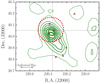 |
Fig. 1. Galaxy overdensity BOSS1441 at z = 2.32 ± 0.02 (Cai et al. 2017a). The density contours (green) for LAEs are shown in steps of 0.1 galaxies per arcmin2, with the inner density peak of 1.0 per arcmin2. The density contours are shown with increasing thickness for increasing galaxy number density. The brown crosses indicate the positions of known QSOs in the redshift range 2.30 ≤ z < 2.34, and thus likely within the overdensity. We also highlight the position of the ELAN MAMMOTH-1 (dotted crosshair), and the effective area of our SCUBA-2 observations (red dashed contour). |
SCUBA-2 observations around the MAMMOTH-1 nebula.
3. Source extraction and catalogs
To extract the detections from both maps, we proceeded following Chen et al. (2013a). We first extracted sources with a peak signal-to-noise ratio (S/N) > 2 within the effective area of our observations (see Table 1). Specifically, our algorithm for source extraction finds the maximum pixel within the selected region, takes the position and the information of the peak, and subtracts a scaled point spread function (PSF) centered at such a position1. The process was iterated until the peak S/N went below 2.0. These sources constituted the preliminary catalogs at 850 and 450 μm. We then cross-checked the two catalogs to find counterparts in the other band. We considered a source as a counterpart if its position at 450 μm lay within the 850 μm beam.
The final catalogs were built by keeping every > 4σ source in the preliminary catalogs, but also every > 3σ source characterized by a > 3σ counterpart in the other band. Overall, we discovered 27 sources at 850 μm and 14 sources at 450 μm. In Tables 2 and 3 we list the information for these sources. Figure 2 shows the final S/N maps at 850 and 450 μm for the targeted field with the discovered sources over-plotted.
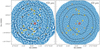 |
Fig. 2. SCUBA-2 S/N maps at 850 μm (top panel) and 450 μm (bottom panel) for the field around the ELAN MAMMOTH-1 (red star). The maps are shown with a linear scale from −4 to 4. The size of both maps is 15′ × 15′. Orange circles are the 27 850 μm detections given in Table 2, and yellow squares are the 14 450 μm detections given in Table 3. For both fields, we indicate the noise contours (black dashed) for levels 1.5, 2, and 3× the central noise (σCN; Table 1). The sizes of the circles and squares correspond to 2× the beam FWHM of their respective wavelength. |
SCUBA-2 850 μm detected sources around the MAMMOTH-1 Nebula.
3.1. Reliability of source extraction
To determine the number of spurious sources that could affect our catalogs, we proceeded as follows. First, we applied the source extraction algorithm to the inverted maps. We found two and one detections at > 4σ at 850 and 450 μm, respectively. Second, we constructed true noise maps, we applied the source extraction algorithm, and checked the number of detections with > 4σ. To obtain true noise maps we used the jackknife resampling technique. Specifically, we subtracted two maps obtained by coadding roughly half of the data for each band. In this way, any real source in the maps is subtracted irrespective of its significance. The residual maps are thus source-free noise maps. To account for the difference in exposure time, we scaled these true noise maps by a factor of  , with t1 and t2 being the exposure time of each pixel from the two maps. These jackknife maps are characterized by a central noise of 0.88 and 5.39 mJy beam−1, respectively, at 850 μm and 450 μm, in agreement with the noise in the science data. By applying the source extraction algorithm to these maps, we found one and four detections at > 4σ at 850 and 450 μm, respectively. We thus expect a similar number of spurious sources in our > 4σ source catalogs.
Further, we tested the number of spurious detections for the 3σ sources identified as having a counterpart in the other bandpass (lower portion of Tables 2 and 3) by using once again the jackknife maps. Specifically, from this maps we extracted sources between 3 and 4σ, and cross-correlated them with the detections in the real data at the other wavelength. We found that none of such spurious sources matched a detection in the real maps. We then repeated the test 1000 times by randomizing the position of the spurious sources within the effective area of our observations. On average we found 0.3 and 0.7 spurious sources at 850 and 450 μm, indicating that sources selected at the > 3σ level in both bandpasses are even more reliable than > 4σ sources selected in only one bandpass.
SCUBA-2 450 μm detected sources around the MAMMOTH-1 Nebula.
Overall these tests suggest that – most likely – the sources at 450 μm without a detection at 850 μm are spurious for our observations. For the sake of completeness, we decided to list all the sources in our catalogs. As it will be clear from our analysis, our conclusions are not affected.
3.2. Completeness tests
We tested at which flux our data can be considered complete. We proceeded as follows. We took the true noise maps introduced in Sect. 3.1, and populated them with mock sources of a given flux and placed at random positions. We then extracted the sources, considering them as recovered if the detection was above 4σ and within the beam area. Specifically, we injected sources with flux from 0.1 to 25.1 mJy (0.1–80.1 mJy) with a step of 0.5 mJy (1.0 mJy) for 850 (450) μm. For each step in flux, we iterated the extraction by introducing 1000 sources. To fully characterize the completeness in the whole extent of the maps, we repeated this procedure for areas of the images characterized by different depths: < 3σCN, 2σCN < σ < 3σCN, 1.5σCN < σ < 2σCN, and σ < 1.5σCN (see Fig. 2). Figure 3 shows the results of the tests. For the whole area with < 3σCN, the 50% completeness is at 5.8 and 37 mJy at 850 and 450 μm, respectively, and the 80% is at 6.8 and 44 mJy, respectively. As expected the central portion of the maps with σ < 1.5σCN has a better sensitivity, with the 50% completeness being around 4.8 and 30 mJy at 850 and 450 μm, respectively, and the 80% being around 5.3 and 32 mJy, respectively.
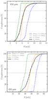 |
Fig. 3. Top: completeness at 850 μm versus flux for different portions of the map, that is, 2σCN < σ < 3σCN, 1.5σCN < σ < 2σCN, σ < 1.5σCN, and < 3σCN (see Fig. 2). Bottom: same as above, but for the 450 μm dataset. |
4. Number counts
In this section we determine the pure source number counts at 850 and 450 μm around the ELAN MAMMOTH-1, and estimate the underlying counts models for each wavelength. A precise measurement of the galaxy number counts needs an accurate estimate of the number of spurious sources contaminating the counts. For this purpose, we followed the procedure in Chen et al. (2013a,b), and used the jackknife maps produced in Sect. 3.1 to assess how many spurious sources affect the counts. As a first step, in Fig. 4 we show the S/N histograms of the true noise maps (orange shading) and the signal maps (blue shading with black edge). The excess signals with respect to the pure noise distribution are from real astronomical sources. On the other hand, the negative excesses are due to the negative troughs of the matched-filter PSF. From these histograms it is well evident that the 450 μm data are less sensitive and more affected by the presence of spurious sources (as already noted in Sect. 3.1).
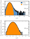 |
Fig. 4. Normalized histograms of the S/N values for the pixels within the portions of the 850 and 450 μm maps characterized by less than three times the central noise. The orange and blue histograms indicate the distributions of the jackknife maps, and of the data, respectively. The jackknife maps represents the pixel noise distributions that dominates at low S/N (see Sect. 3.1 for details). The data (especially at 850 μm) shows excesses at high S/N where sources contribute to the distributions. The matched filter technique introduces residual troughs around bright detections, which are visible here as negative excesses. |
In contrast to what was done with the catalogs in Sect. 3 – where we selected only detections with S/N > 4 or with S/N > 3 at both wavelengths – we lowered our detection threshold to 2σ. Indeed, as the positional information is not relevant for number counts analyses, the detection threshold can be lowered to explore statistically significant positive excesses (e.g., Chen et al. 2013b). We thus used the preliminary catalogs produced in Sect. 3, and additionally ran the source extraction algorithm on the true noise maps down to S/N = 2.
The pure source differential number counts are then obtained as follows. First, for each extracted source in the signal map we calculated the number density by inverting the detectable area, which is the portion of the field of view with noise level low enough to allow the detection of the source. Second, we obtained the raw number counts by summing up the number densities of the sources within each flux bin. Finally, to get to the pure source differential number counts, we subtracted the number counts similarly obtained from the true noise maps, if any, from the counts obtained from the signal maps. Figure 5 shows the obtained pure source differential number counts (black data points) for both 850 (top panel) and 450 μm (lower panel).
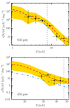 |
Fig. 5. Pure source differential number counts (black data-point) at 850 and 450 μm around the ELAN MAMMOTH-1 compared to the simulated mean counts (red dashed line). The yellow shadings represent the 90% confidence range obtained from 500 realizations of the blue dot-dashed curves. The blue dot-dashed curves are the final adopted underlying models for the Monte Carlo simulations (see Sect. 4), and represent the true number counts. The dashed vertical lines indicate the mean 4σ within the effective area. The horizontal errorbars for the data-points indicate the width of each flux bin. |
To obtain the underlying counts models, we ran Monte Carlo simulations following, for example, Chen et al. (2013a,b). First, we created a simulated image by randomly injecting mock sources onto the jackknife maps. The mock sources were drawn from an assumed model and convolved with the PSFs. For the counts models we used a broken power law of the form
 (1)
(1)
and started from a fit to the observed counts. As faintest fluxes for our models, we used the fluxes at which the integrated flux density agrees with the values for the extragalactic background light (EBL; e.g., Puget et al. 1996).
After obtaining a mock map, we ran the source extraction algorithm and computed the number counts in exactly the same way as done with the real data. We then calculated the ratio between the recovered counts and the input model, which reflects the Eddington bias (Eddington 1913), and then applied this ratio to the observed counts to correct for this bias. A χ2 fit is performed to the corrected observed counts using the broken power law to get the normalization and power-law indices, which are then used in the next iteration. This iterative process was terminated once the input model agreed with the corrected counts at the 1σ level. Given the low number of data-points at 450 μm, we only fitted the normalization and the bright-end slope at this wavelength. We fixed S0 and α to the values in Chen et al. (2013b).
To test the reliability of our results, we then created 500 realizations of simulated maps using as input the model curves determined through the Monte Carlo simulations, and calculated the pure source number counts for each of them. In Fig. 5 we show the results of the Monte Carlo simulations and compare them to the data. We give the derived underlying counts models (blue dot-dashed lines), the mean counts (red dashed lines), and the 90% confidence range of the 500 realizations (yellow). The 500 realizations well match the pure source number counts within the uncertainties. We can then apply the ratio between the mean number counts and the input model to correct our data, and thus obtain the true differential number counts (see Sect. 7.1). Table 4 summarizes the parameters of the obtained underlying count models at both 850 and 450 μm.
5. Flux boosting estimates
With the Monte Carlo simulations we found a systematic flux boost, which we characterized by comparing the flux of the injected mock sources with the detections. In particular, we selected the brightest input source located within the beam area of each of the > 3σ recovered sources, and computed the flux ratio. In Fig. 6 we show this test as a function of S/N for both wavelengths. We plot the mean (red) and the median (yellow) values of the flux boosting, together with the 1σ ranges (blue) relative to the mean values. At S/N = 4, the estimated median flux boosting is 2.0 and 1.5 at 450 and 850 μm, respectively. These values are in agreement within the uncertainties with similar previous studies conducted with SCUBA-2 (e.g., Casey et al. 2013; Chen et al. 2013a). We then corrected the observed fluxes for the catalogs obtained in Sect. 3 using the median curves, and listed the de-boosted fluxes in Tables 3 and 2. This flux boost is usually found in previous SCUBA studies (e.g., Wang et al. 2017) and it is ascribed to the Eddington bias (Eddington 1913).
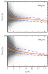 |
Fig. 6. Ratio between the fluxes of the detected sources and the injected sources from the 500 realizations of the estimated underlying counts models (Sect. 4) as a function of the S/N of the detections. The gray dots are ∼100 000 simulated data-points. We show the mean (red) and median (yellow) values of the flux ratio in different S/N bins. The blue dashed curves enclose the 1σ range relative to the mean curve. The test is shown for both 850 (top) and 450 μm (bottom). |
6. Positional uncertainties
Using the same Monte Carlo simulations and the same algorithm to find counterparts in the injected and recovered catalogs, we can estimate the positional offset between the location of the injected and the recovered sources. Figure 7 shows this test at both 450 and 850 μm. At S/N ≲ 5, there is a large scatter, suggesting positional uncertainties of the order of ≳1.7 and ≳2.2 arcsec, respectively, for 450 and 850 μm. At larger S/N the uncertainty is lower, down to 1 arcsec for sources as strong as the brightest objects in our 850 μm catalog (S/N ∼ 16). At 450 μm – characterized by a ∼1.5× smaller beam – the positional uncertainties are slightly smaller. These results agree well – within the uncertainties – with the predicted positional offset based on the LABOCA ECDFS Submm Survey (LESS) sample (dashed black line; Eq. (B22) in Ivison et al. 2007). Based on this test, we can then assign the mean value of the offsets as positional uncertainty to the detections listed in Tables 3 and 2.
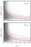 |
Fig. 7. Positional offset between the detected sources and the injected sources from the 500 realizations of the estimated underlying counts models (Sect. 4) as a function of the S/N of the detections. The gray dots are ∼100 000 simulated data-points. We show the mean (red) and median (yellow) values of the positional offsets in different S/N bins. The blue dashed curves enclose the 1σ range relative to the mean curve. The test is shown for both 850 (top) and 450 μm (bottom). The dot-dashed black lines indicate the predictions from Ivison et al. (2007) based on the LESS sample. |
7. Results
7.1. True number counts
Figure 8 presents the corrected differential and cumulative number counts at both 450 and 850 μm for the effective area of our observations, together with the derived underlying broken power-law (bpl) models (blue dot-dashed lines). As explained in Sect. 4, these true number counts have been obtained by dividing the pure source counts by the ratio between the mean number counts and the input models. We list the values of our corrected data-points in Table 5.
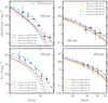 |
Fig. 8. Comparison of the SCUBA-2 MAMMOTH-1 differential number counts at 850 μm (top left) and 450 μm (top right), and the cumulative number counts at 850 μm (bottom left) and 450 μm (bottom right) with respect to estimates for blank fields in the literature (Chen et al. 2013b; Casey et al. 2013; Geach et al. 2013, 2017; Wang et al. 2017; Zavala et al. 2017). The black filled symbols are the corrected counts following our Monte Carlo simulations (see Sect. 4), and the blue dot-dashed curves are our true number counts curves from Table 4. When comparing to blank fields, our data for the MAMMOTH-1 field thus show higher counts at 850 μm, but not at 450 μm. |
True number counts at 450 and 850 μm.
We then compare our data-points with the most comprehensive literature studies for blank fields at both 450 and 850 μm (Chen et al. 2013b; Casey et al. 2013; Geach et al. 2013, 2017; Wang et al. 2017; Zavala et al. 2017). In Fig. 8 we plot the fit – Schechter (Sc.) or broken power-law (bpl)2 – from those works. Our 450 μm data agree well with these literature curves3, while the 850 μm data-points are above these current expectations for blank fields. Especially the more robust data at about 5 and 7 mJy clearly suggest the presence of higher number counts with respect to the literature values.
To quantify this overdensity of counts at 850 μm, we fit our corrected differential number counts with the functions from each of the literature works allowing only the normalization to vary. The difference in counts is then estimated through the ratio between the normalizations. Specifically,
-
Chen et al. (2013b) quoted a best fit with a broken power-law function of the form shown in Eq. (1), with4
 mJy−1 deg−2, S0 = 6.21 mJy, α = 2.27, β = 3.71;
 -
Casey et al. (2013) and Geach et al. (2017) reported a Schechter function of the form
 (2)
(2)with N0 = (3.3 ± 1.4)×103 deg−2, S0 = 3.7 mJy, γ = 1.4, and5N0 = 4550 ± 546 deg−2, S0 = 3.40 ± 0.21 mJy, γ = 1.97 ± 0.08, respectively;
-
Zavala et al. (2017) preferred a Schechter function of the form
 (3)
(3)with N0 = 8300 ± 300 deg−2, S0 = 2.3 mJy, γ = 2.6 for all their data.
We show the results of the fit with free normalizations N0 in Fig. 9, and we list in Table 6 the ratio between the derived normalizations needed to match our data and the literature values. From these ratios it is clear that the probed effective area is indeed overdense with respect to blank fields. On average, around the ELAN MAMMOTH-1 there are 4.0 ± 1.3 times more counts than in blank fields. In this mean estimate we do not include the ratio with respect to Zavala et al. (2017) because this work does not cover effectively the sources bright-end (their last bin is at 4.9 mJy), probably biasing their fit. We do, however, report the comparison with this work for completeness.
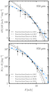 |
Fig. 9. Top: fit of the SCUBA-2 MAMMOTH-1 true differential number counts at 850 μm using the functions given in literature works for blank fields (Chen et al. 2013b; Casey et al. 2013; Zavala et al. 2017; Geach et al. 2017) with N0 free to vary. Bottom: SCUBA-2 MAMMOTH-1 true cumulative number counts at 850 μm compared to the fit models obtained in the top panel. In both panels, the blue dot-dashed curve is our true number counts curve from Table 4. All the literature models need a significant increase of their normalization parameter N0 to fit our data at 850 μm, revealing that the covered effective area is overdense with respect to blank fields. We list the values in Table 6. |
Overdensity estimates at 850 μm from the fit to our true differential number counts with literature functions for blank fields.
7.2. Position of the catalog sources within the LAE overdensity
Even though the association to the BOSS1441 overdensity of the sources listed in the SCUBA-2 catalogs has to be confirmed spectroscopically, we can still search for LAE counterparts to our submillimeter detections, if any. In Fig. 10, we show the location of the 450 (yellow squares) and 850 μm (blue circles, with fluxes) catalog sources along with (i) the position of known LAEs (black circles; Cai et al. 2017a), (ii) the position of known QSOs at 2.30 ≤ z < 2.34 (brown crosses; Cai et al. 2017a), and (iii) the LAEs’ density contours (green; Cai et al. 2017a). From this figure it is clear that only two sources out of the 27 850 μm detections could be considered to be possibly associated with an LAE from the catalogue of Cai et al. (2017a). These two sources (highlighted in orange) are (i) MAM-850.14 close to the ELAN MAMMOTH-1 (see Sect. 8.2 for a discussion), and (ii) MAM-850.16 close to an LAE at RA = 220.3906 and Dec = 40.0286, with rest-frame equivalent width EW0 = 25.16±0.01 Å, which is actually a z ≃ 2.3 QSO.
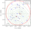 |
Fig. 10. Comparison of the location of the known LAEs within the galaxy overdensity BOSS1441 and the SCUBA-2 submillimeter detections in our field of view (red; as in Fig. 1). We indicate the position of the LAEs (black circles), QSOs in the redshift range 2.30 ≤ z < 2.34 (brown crosses), detections at 850 μm (blue circles; the number indicates the observed flux in unit of mJy; the size of circles equals the FWHM), and detection at 450 μm (yellow squares; the size of symbol equals the FWHM). As in Fig. 1 we show the density contours (green) for LAEs in steps of 0.1 galaxies per arcmin2, with the inner density peak of 1.0 per arcmin2. We also highlight the position of the ELAN MAMMOTH-1 (dotted crosshair), and the field of view of our SCUBA-2 observations for 3× the central noise (red dashed contour). Overall, the LAEs and submillimeter sources are not associated. Only the ELAN MAMMOTH-1 and an additional LAE can be considered as counterparts of a submillimeter detection, MAM-850.14 and MAM-850.16 respectively (highlighted as orange diamonds). Intriguingly the brightest submillimeter detections coincide with the peak of the BOSS1441 overdensity. |
The other 25 LAEs lay at a separation greater than the 850 μm beam from any of our detections. Given the large offsets, the positional uncertainties presented in Sect. 6 do not affect the lack of association between LAEs and our submillimeter detections. If future follow-up studies confirm the association of most of the SCUBA-2 sources with the BOSS1441 overdensity, the lack of submillimeter flux at the location of LAEs is consistent with the usual finding that most of the strongly Lyα emitting galaxies are relatively devoid of dust (e.g., Ono et al. 2010; Hayes et al. 2013; Sobral et al. 2018).
In addition, the brightest detections at 850 μm, MAM-850.1 and MAM-850.2 ( mJy and
  mJy), lay intriguingly close to the peak of the LAEs’ overdensity. Their observed ratios between 450 and 850 μm suggest that these two bright detections are unlikely to be low redshift sources. Therefore, they probably are associated with the protocluster given the rare alignment with the peak of the LAEs’ overdensity.
8. Discussion
8.1. BOSS1441: A rich and diverse protocluster
In the previous sections we have demonstrated the presence of an approximately four times higher density fluctuation compared to blank fields at 850 μm. In addition, we found that the brightest of our detections are located at the peak of the LAEs’ overdensity. This unique alignment suggest that most of the SCUBA-2 detections are likely associated with the BOSS1441 overdensity (and the ELAN MAMMOTH-1), rather than being intervening.
To test this, we searched the available multiwavelength catalogs and built the spectral energy distributions (SEDs) for all the sources in our sample. We thus looked for counterparts in the AllWISE Source Catalog6 (Wright et al. 2010) produced using the Wide-Field Infrared Survey Explorer (WISE) bands at 3.4, 4.6, 12.1, 22.2 μm (W1, W2, W3, W4), and in the Faint Images of the Radio Sky at Twenty-cm (FIRST) Survey at 1.4 GHz (Becker et al. 1994). This portion of the sky has not been covered by the Herschel telescope and thus our SCUBA-2 observations are key in covering the far-infrared portion of the SED. To match the different catalogs, we looked for counterparts within an 850 μm beam, and selected the closest source. We found that eight of our detections have a counterpart in AllWISE, while none have been detected in FIRST down to the catalog detection limit at each source position (∼0.95 mJy). To estimate the likelihood of false match for the WISE counterparts, we use the p-value as defined in Downes et al. (1986),
 (4)
(4)
where n is the AllWISE source density within the effective area, n ≃ 0.00134 sources/arcsec2, and θ is the angular separation between the AllWISE source and the SCUBA-2 detection7. A value of p < 0.05 usually makes a counterpart reliable (e.g., Ivison et al. 2002; Chen et al. 2016), while 0.05 < p < 0.1 makes it tentative (e.g., Chapin et al. 2009). Of the eight counterparts we found that only four are robust, MAM-850.8, MAM-850.18, MAM-850.26 and MAM-850.27, while the others are tentative. However, we have shown in Sect. 7.2 that MAM-850.16 is likely associated with a quasar at z = 2.30. As the quasar is detected by WISE and no other close WISE detections are present, we consider this match secure. Further, the lack of available radio and/or high resolution submillimeter data prevents us from performing a robust identification of counterparts in our recently obtained U, V, and i band images with the Large Binocular Telescope (LBT; Cai et al. 2017a) and in our J, H, and K band images obtained with the United Kingdom Infrared Telescope (UKIRT; Xu et al., in prep.). We summarize the sources with multiwavelength detections in Table A.1, and display for illustration purposes the SEDs of the five sources with robust counterparts in AllWISE in Fig. A.1.
We leave a detailed classification of our detections to future studies encompassing the whole protocluster extent, and better covering the electromagnetic spectrum. However, we used the average SED template for SMGs obtained from 99 sources in the ALESS (ALMA LESS) survey (da Cunha et al. 2015)8 to compute a rough estimate for the far-infrared (FIR) luminosity LFIR for each source assuming they are all SMGs at z = 2.32 (redshift of BOSS1441). After normalizing the SED template to our SCUBA-2 observations, we found LFIR ≥ 4.8 × 10¹² L⊙ for each of the sources9.
Next, we compared the volume density implied by our observations with expectations from the current luminosity function of SMGs. Assuming the effective area of our observations (∼336.9 Mpc2) and the distance interval spanned in redshift by the protocluster (z = 2.3 − 2.34; ∼34.9 Mpc−3), the comoving volume targeted by our observations is about 11 800 Mpc3. If all (75%) of the detections at 850 μm belong to the protocluster, their volume density would then be 2.3 × 10⁻³ Mpc−3 (1.7 × 10⁻³ Mpc−3). These values are a factor of > 30 above the volume density expected from the current luminosity function of SMGs with LFIR ≥ 4.8 × 10¹² L⊙ (∼5 × 10⁻⁵ Mpc−3; Casey et al. 2014). Therefore, BOSS1441 is a potentially SMG-rich volume.
We further noticed that the two brightest sources, MAM-850.1 and MAM-850.2, seem to depart from the templates at 850 μm, showing higher fluxes than expected. This deviation could be explained by allowing a different (higher) redshift, or most probably by the fact that single-dish submillimeter sources as bright as MAM-850.1 and MAM-850.2 are usually a blend of ≥2 SMGs once observed with interferometers (Karim et al. 2013; Simpson et al. 2015). This explanation is compelling as the two sources sit at the peak of the overdensity. They could thus be groups of interacting galaxies, pinpointing the core of the protocluster.
Extremely compact (20″ − 40″) protocluster cores made of several (> 10) starbursting galaxies at z ∼ 4 have been recently discovered by Miller et al. (2018) and Oteo et al. (2018). These structures have a global LFIR ≈ 1014 L⊙ (Miller et al. 2018). The BOSS1441 protocluster might thus have similar, but scaled down central structures. We can compare this central portion of the overdensity with other known protoclusters at z ∼ 2 (Dannerbauer et al. 2014; Casey et al. 2015; Kato et al. 2016). These studies found that spheres with 1 Mpc radius centered at the protocluster core enclose a star formation rate density of SFRD ∼ 1000 − 1500 M⊙ yr−1 Mpc−3. Following the approach in those works, we centered a 1 Mpc sphere at the position of MAM-850.2, which is the closest SMG to the peak of the LAE overdensity. Within this sphere we potentially found six detections (MAM-850.1, MAM-850.2, MAM-850.12, MAM-850.14, MAM-850.16, MAM-850.21), which add up to a total star formation rate of SFR = 9100 M⊙ yr−1, translating to SFRD ≈ 2200 M⊙ yr−1 Mpc−3 after dividing by the sphere volume10. As our detections are candidate SMGs, this value represents an upper limit. Subtracting the field average value as done in Kato et al. (2016) for z = 2.3, and assuming that only 75% of our detections are within the sphere, we obtained SFRD ≈ 1200 M⊙ yr−1 Mpc−3. We conservatively conclude that  yr−1 Mpc−3, with the lower limit given by the very unlike case that none of the detections (apart the ELAN MAMMOTH-1 counterpart) are within the sphere. This SFRD value is in agreement with values for protoclusters in the literature (e.g., see Fig. 5 in Kato et al. 2016).
Spectroscopic and interferometric follow-ups are needed to confirm the redshift of our sources, and to unveil their nature. Our analysis, however, suggests that BOSS1441 is a rich protocluster hosting several LAEs, one ELAN, and likely several SMGs.
8.2. The counterpart of the ELAN MAMMOTH-1
Cai et al. (2017b) reported the presence of a continuum source at z = 2.319 ± 0.004, named source B, and of a z = 0.16 AGN, both at the location of the peak of the ELAN MAMMOTH-1. Source B has been invoked as the powering source of the extended Lyα emission. At a separation of 4.58″ from source B and at 2.75″ from the z = 0.16 AGN, our SCUBA-2 observations resulted in a bright detection at 850 μm, MAM-850.14, with flux density of f850 = 4.57 ± 0.93 mJy ( mJy), and a 3σ upper limit of f450 < 16.65 mJy at 450 μm. The non-detection at 450 μm suggests that the emission at 850 μm is associated with the z = 2.319 source. Indeed, a z = 0.16 AGN with such a detection at 850 μm should have a much brighter dust thermal emission at 450 μm. Specifically, if we assume a modified black body for optically thin thermal dust emission, a dust temperature of Tdust = 45 K, and the largely used emissivity index β = 1.5 (e.g., Casey 2012), we find that a z = 0.16 AGN should have f450 = 35.3 mJy (or 21.8 mJy for the deboosted flux). These fluxes would be detected at high significance (≳4σ) even in our shallow 450 μm data at the location of the ELAN MAMMOTH-1.
To constrain the nature of source B, we compiled all its data available from the literature, and compared them to known SED. We summarize all the available observations in Table 711, while we plot them in Fig. 11.
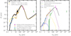 |
Fig. 11. SED for the source powering the ELAN MAMMOTH-1 at z = 2.319 (source B in Cai et al. 2017b). The data-points are from LBT/LBC imaging and UKIRT/WIRCAM (Cai et al. 2017b and Xu et al. in prep.; blue), AllWISE source catalog (Wright et al. 2010; orange), our SCUBA-2 observations (magenta), and the FIRST survey (Becker et al. 1994; green). Left panel: data-points in comparison to the SED of M 82 (Silva et al. 1998; black line), of the average ALESS SMGs (dashed brown line), and of the average ALESS SMGs with AV < 1 (da Cunha et al. 2015; yellow), best fitting our data-points for z = 2.319. The best agreement is found for the M82 template, but the W3 data-point is underestimated. Right panel: data-points in comparison to the best fit of AGNfitter (gray line), together with the individual components: hot dust emission (purple), cold dust emission (green), stellar emission (yellow), and the emission from the accretion disk (blue). The hot dust contribution allows a better fit to the data. |
Data for source B, counterpart of the MAMMOTH-1 ELAN.
To compare these data-points to known SEDs, we fixed the redshift of the source to the redshift z = 2.319 determined from the He II line emission (Cai et al. 2017b), and we fit the data leaving the normalization free. We first took into consideration the average SED for SMGs obtained from the 99 sources in ALESS (da Cunha et al. 2015), and all the available average SEDs from that publication. The left panel of Fig. 11 shows this test, highlighting the shortage of emission at the WISE bands for these SED templates (we plot only two to avoid confusion) in comparison to the source B’s data-points. None of the average templates in da Cunha et al. (2015) match the W1,W2,W3 data-points, with the SED with AV < 1 (yellow) giving the closer values, though differing still significantly. We then follow the same procedure with the template SED of the local starburst galaxy M 82 (Silva et al. 1998; solid black line in Fig. 11). This template gives a significantly better match to the observations, with only the W3 data-point underestimated. Most likely a hotter dust component powered by an AGN (e.g., Silva et al. 2004; Fritz et al. 2006) would allow a better match of the data of source B. Indeed Cai et al. (2017b) demonstrate that only hard-ioninzing sources – most likely an AGN or a wind – could power the He II and C IV emission in this object.
To test this interpretation further, we used the publicly available SED fitting code, AGNfitter (Calistro Rivera et al. 2016), which adopts a fully Bayesian Markov Chain Monte Carlo method to model the SEDs of galaxies and AGN. AGNfitter fits simultaneously the submillimeter to UV photometry, decomposing the SED into four physically motivated components: the AGN accretion disk emission (Big Blue Bump), the hot dust emission from the obscuring structure around the accretion disk (torus), the cold dust emission from star-forming regions, and the stellar populations of the host galaxy12. Details on the specific models are presented by Calistro Rivera et al. (2016) and references therein. The right panel of Fig. 11 shows the best fit (in gray) produced by AGNfitter, with each component highlighted by a different color. The W3 data-point is now well covered by a composition of the AGN-powered hot dust, star emission, and star-formation-powered cold dust.
This analysis thus suggests that source B is an enshrouded strong starbursting galaxy, likely hosting an obscured AGN. Using the output from AGNfitter, we can separate the far-infrared (FIR) luminosity LFIR (rest-frame 8–1000 μm) due to the AGN and to star formation (SF). We find  and
and  , respectively. Source B thus meets the generally used criteria to define an ultraluminous infrared galaxy (ULIRG; L8 − 1000μm > 1012 L⊙; e.g., Sanders & Mirabel 1996). Following the classical conversion in Kennicutt (1998) and considering only the star-formation-powered emission, one would then obtain a star formation rate of SFR
  yr−1.
yr−1.
In agreement with the observations and analysis in Cai et al. (2017b), our analysis thus suggests a strong similarity between the source B embedded within the ELAN MAMMOTH-1 and the ULIRG sample hosting AGN activity in Harrison et al. (2012). Source B – with its obscured AGN and starburst – can thus easily power the surrounding ELAN, and thus the outflow resulting in the velocity offset of 700 km s−1 between the two spectral components in Lyα, He II, and C IV (Cai et al. 2017b). The very broad [O III] emission presented for the targets in Harrison et al. (2012), however, extends to lower distances (15 kpc) with respect to the rest-frame UV lines seen in the ELAN MAMMOTH-1 (≳30 kpc; Cai et al. 2017b). As the ELAN MAMMOTH-1 hosts an ULIRG we thus expect to see broad [O III] emission in its central portion down to similar depths.
Finally, AGNfitter estimated the stellar mass of source B to be log . By inverting the halo mass Mhalo–Mstar relation in Moster et al. (2013), we derived that, if source B is a central galaxy, the ELAN MAMMOTH-1 is hosted by a very massive halo of log
 . Given the large uncertainties, this result has to be confirmed. However, it certainly highlights the peculiarity of the halo hosting the ELAN MAMMOTH-1, indicating that it sits at the high-mass end of the halo population at this redshift. We further note that the stellar mass of source B is intriguingly close to current estimates for the stellar mass of host galaxies of HzRGs (log(Mstar/M⊙)≃11 − 11.5; Seymour et al. 2007; De Breuck et al. 2010). HzRGs are currently thought to reside in massive halos of mass log(Mhalo/M⊙)≈13 (e.g., Stevens et al. 2003). The halo hosting the ELAN MAMMOTH-1 could thus be similarly massive or exceed such halos.
9. Summary
We are currently conducting a survey of all the known ELANe (Cantalupo et al. 2014; Hennawi et al. 2015; Cai et al. 2017b; Arrigoni Battaia et al. 2018) with the JCMT and APEX telescopes to assess the presence of starburst activity in these systems and their environments. In this work we focused on the SCUBA-2/JCMT data at 450 and 850 μm obtained for an effective area of ∼127 arcmin2 around the ELAN MAMMOTH-1 at z = 2.319 (Cai et al. 2017b), and thus targeting the known peak area of the LAE overdensity BOSS1441 (Cai et al. 2017a). Thanks to this dataset we found that:
-
the 850 μm source counts are 4.0 ± 1.3 times higher than in blank fields (Chen et al. 2013b; Casey et al. 2013; Geach et al. 2017), confirming also in obscured tracers the presence of an overdensity. Intriguingly, the two brightest submillimeter detections, MAM-850.1 and MAM-850.2, are located at the peak of the LAE overdensity, possibly pinpointing the core of the protocluster and multiple mergers and/or interactions (e.g., Miller et al. 2018). The association of the discovered submillimeter sources with BOSS1441 needs, however, a spectroscopic confirmation.
-
the continuum source at the center of the ELAN MAMMOTH-1, source B (Cai et al. 2017b), is associated to a strong detection at 850 μm, MAM-850.14, with flux density of f850 = 4.6 ± 0.9 mJy (
 mJy) and a 3σ upper limit of f450 < 16.6 mJy at 450 μm. Together with the data from the literature, the SED of source B agrees with a strongly starbursting galaxy hosting an obscured AGN, and having an FIR luminosity of
  . Source B is thus an ULIRG with a star formation rate of SFR
  yr−1 assuming the classical Kennicutt (1998) calibration. Such a source – containing both an AGN and a violent starburst – is able to power the hard photoionization plus outflow scenario depicted in Cai et al. (2017b).
The acquisition of wide-field multiwavelength data (X-ray, UV, optical, submillimeter, radio) is key in painting a coherent and detailed picture of a protocluster, and ultimately understanding the assembly of massive galaxies within the cosmic nurseries of the soon-to-be large clusters. The results of this pilot project are encouraging and reflect the importance of such a multiwavelength approach in fully comprehending the ELAN phenomenon and the environment in which they reside.
As PSFs for our observations, we adopt the PSFs at 850 and 450 μm generated by Chen et al. (2013b; see their Fig. 2).
If a work presented both functions for their fits, we selected their Schechter fit. Our results do not depend on this choice.
We remind the reader that – as already noted in Casey et al. (2013) – the Eq. (1) of Geach et al. (2013) should be written as dN/dS = (N′/S′)(S/S′)1 − αexp(−S/S′), and the best-fitting parameter N′ for this 450 μm data should be quoted as N′ = 4900 ± 1040 deg−2 mJy−1 rather than N′ = 490 ± 1040 deg−2 mJy−1.
For all the fits in the literature, we report only the errors on the parameter N0.
Geach et al. (2017) only showed a Schechter fit to their data in their Fig. 15. Here we thus report the values for a Schechter fit to their data.
As the positional uncertainty is small for the 450 μm band, for our sources we adopt the coordinates at 450 μm if available.
da Cunha et al. (2015) provides average SEDs made in bins of redshifts, observed ALMA 870 μm flux, average V-band attenuation AV, total dust luminosity (http://astronomy.swinburne.edu.au/~ecunha/ecunha/SED_Templates.html).
We estimated the FIR luminosity LFIR for each source as frequently done by integrating the luminosity in the rest-frame range 8–1000 μm.
We convert LFIR to SFR using the classical conversion in Kennicutt (1998).
The U, V, i-band photometry here reported is slightly (within errors) different from Cai et al. (2017b) because of the image degradation applied to the data to match the UKIRT observations (Xu et al., in prep.).
AGNfitter does not currently cover the radio portion of the spectrum. This does not affect our results as we do not have stringent limits for the radio wavelengths.
Acknowledgments
We thank the referee Yuichi Matsuda for his careful reading of the manuscript. The James Clerk Maxwell Telescope is operated by the East Asian Observatory on behalf of The National Astronomical Observatory of Japan; Academia Sinica Institute of Astronomy and Astrophysics; the Korea Astronomy and Space Science Institute; the Operation, Maintenance, and Upgrading Fund for Astronomical Telescopes and Facility Instruments, budgeted from the Ministry of Finance (MOF) of China and administrated by the Chinese Academy of Sciences (CAS), as well as the National Key R&D Program of China (No. 2017YFA0402700). Additional funding support is provided by the Science and Technology Facilities Council of the United Kingdom and participating universities in the United Kingdom and Canada. This publication makes use of data products from the Wide-field Infrared Survey Explorer, which is a joint project of the University of California, Los Angeles, and the Jet Propulsion Laboratory/California Institute of Technology, and NEOWISE, which is a project of the Jet Propulsion Laboratory/California Institute of Technology. WISE and NEOWISE are funded by the National Aeronautics and Space Administration. M.F. acknowledges support by the Science and Technology Facilities Council [grant number ST/P000541/1]. This project has received funding from the European Research Council (ERC) under the European Union’s Horizon 2020 research and innovation program (grant agreement No. 757535). I.R.S. acknowledges support from the ERC Advanced Grant DUSTYGAL (321334) and STFC (ST/P000541/1). Y.Y.’s research was supported by Basic Science Research Program through the National Research Foundation of Korea (NRF) funded by the Ministry of Science, ICT & Future Planning (NRF-2016R1C1B2007782). The authors wish to recognize and acknowledge the very significant cultural role and reverence that the summit of Mauna Kea has always had within the indigenous Hawaiian community. We are most fortunate to have the opportunity to conduct observations from this mountain.
References
- Alaghband-Zadeh, S., Chapman, S. C., Swinbank, A. M., et al. 2012, MNRAS, 424, 2232 [NASA ADS] [CrossRef] [Google Scholar]
- Arrigoni Battaia, F., Hennawi, J. F., Prochaska, J. X., & Cantalupo, S. 2015a, ApJ, 809, 163 [NASA ADS] [CrossRef] [Google Scholar]
- Arrigoni Battaia, F., Yang, Y., Hennawi, J. F., et al. 2015b, ApJ, 804, 26 [NASA ADS] [CrossRef] [Google Scholar]
- Arrigoni Battaia, F., Prochaska, J. X., Hennawi, J. F., et al. 2018, MNRAS, 473, 3907 [NASA ADS] [CrossRef] [Google Scholar]
- Becker, R. H., White, R. L., & Helfand, D. J. 1994, in Astronomical Data Analysis Software and Systems III, eds. D. R. Crabtree, R. J. Hanisch, & J. Barnes, ASP Conf. Ser., 61, 165 [NASA ADS] [Google Scholar]
- Cai, Z., Fan, X., Bian, F., et al. 2017a, ApJ, 839, 131 [NASA ADS] [CrossRef] [Google Scholar]
- Cai, Z., Fan, X., Yang, Y., et al. 2017b, ApJ, 837, 71 [NASA ADS] [CrossRef] [Google Scholar]
- Cai, Z., Hamden, E., Matuszewski, M., et al. 2018, ApJ, 861, L3 [NASA ADS] [CrossRef] [Google Scholar]
- Calistro Rivera, G., Lusso, E., Hennawi, J. F., & Hogg, D. W. 2016, ApJ, 833, 98 [NASA ADS] [CrossRef] [Google Scholar]
- Cantalupo, S., Arrigoni-Battaia, F., Prochaska, J. X., Hennawi, J. F., & Madau, P. 2014, Nature, 506, 63 [NASA ADS] [CrossRef] [Google Scholar]
- Casey, C. M. 2012, MNRAS, 425, 3094 [Google Scholar]
- Casey, C. M. 2016, ApJ, 824, 36 [NASA ADS] [CrossRef] [EDP Sciences] [Google Scholar]
- Casey, C. M., Chen, C.-C., Cowie, L. L., et al. 2013, MNRAS, 436, 1919 [NASA ADS] [CrossRef] [Google Scholar]
- Casey, C. M., Narayanan, D., & Cooray, A. 2014, Phys. Rep., 541, 45 [NASA ADS] [CrossRef] [Google Scholar]
- Casey, C. M., Cooray, A., Capak, P., et al. 2015, ApJ, 808, L33 [NASA ADS] [CrossRef] [Google Scholar]
- Chapin, E. L., Pope, A., Scott, D., et al. 2009, MNRAS, 398, 1793 [NASA ADS] [CrossRef] [Google Scholar]
- Chapin, E. L., Berry, D. S., Gibb, A. G., et al. 2013, MNRAS, 430, 2545 [NASA ADS] [CrossRef] [Google Scholar]
- Chen, C.-C., Cowie, L. L., Barger, A. J., et al. 2013a, ApJ, 762, 81 [NASA ADS] [CrossRef] [Google Scholar]
- Chen, C.-C., Cowie, L. L., Barger, A. J., et al. 2013b, ApJ, 776, 131 [NASA ADS] [CrossRef] [Google Scholar]
- Chen, C.-C., Smail, I., Swinbank, A. M., et al. 2015, ApJ, 799, 194 [NASA ADS] [CrossRef] [Google Scholar]
- Chen, C.-C., Smail, I., Ivison, R. J., et al. 2016, ApJ, 820, 82 [NASA ADS] [CrossRef] [Google Scholar]
- da Cunha, E., Walter, F., Smail, I. R., et al. 2015, ApJ, 806, 110 [NASA ADS] [CrossRef] [Google Scholar]
- Dannerbauer, H., Kurk, J. D., De Breuck, C., et al. 2014, A&A, 570, A55 [NASA ADS] [CrossRef] [EDP Sciences] [Google Scholar]
- De Breuck, C., Seymour, N., Stern, D., et al. 2010, ApJ, 725, 36 [NASA ADS] [CrossRef] [Google Scholar]
- Dempsey, J. T., Friberg, P., Jenness, T., et al. 2013, MNRAS, 430, 2534 [Google Scholar]
- Dijkstra, M., & Loeb, A. 2009, MNRAS, 400, 1109 [NASA ADS] [CrossRef] [Google Scholar]
- Downes, A. J. B., Peacock, J. A., Savage, A., & Carrie, D. R. 1986, MNRAS, 218, 31 [NASA ADS] [CrossRef] [Google Scholar]
- Eddington, A. S. 1913, MNRAS, 73, 359 [Google Scholar]
- Engel, H., Tacconi, L. J., Davies, R. I., et al. 2010, ApJ, 724, 233 [NASA ADS] [CrossRef] [Google Scholar]
- Fritz, J., Franceschini, A., & Hatziminaoglou, E. 2006, MNRAS, 366, 767 [Google Scholar]
- Fu, H., Cooray, A., Feruglio, C., et al. 2013, Nature, 498, 338 [NASA ADS] [CrossRef] [Google Scholar]
- Geach, J. E., Chapin, E. L., Coppin, K. E. K., et al. 2013, MNRAS, 432, 53 [NASA ADS] [CrossRef] [Google Scholar]
- Geach, J. E., Narayanan, D., Matsuda, Y., et al. 2016, ApJ, 832, 37 [NASA ADS] [CrossRef] [Google Scholar]
- Geach, J. E., Dunlop, J. S., Halpern, M., et al. 2017, MNRAS, 465, 1789 [NASA ADS] [CrossRef] [Google Scholar]
- Harrison, C. M., Alexander, D. M., Swinbank, A. M., et al. 2012, MNRAS, 426, 1073 [NASA ADS] [CrossRef] [Google Scholar]
- Hayes, M., Östlin, G., Schaerer, D., et al. 2013, ApJ, 765, L27 [NASA ADS] [CrossRef] [Google Scholar]
- Hennawi, J. F., Prochaska, J. X., Cantalupo, S., & Arrigoni-Battaia, F. 2015, Science, 348, 779 [NASA ADS] [CrossRef] [PubMed] [Google Scholar]
- Holland, W. S., Bintley, D., Chapin, E. L., et al. 2013, MNRAS, 430, 2513 [NASA ADS] [CrossRef] [Google Scholar]
- Humphrey, A., Zeballos, M., Aretxaga, I., et al. 2011, MNRAS, 418, 74 [NASA ADS] [CrossRef] [Google Scholar]
- Hung, C.-L., Casey, C. M., Chiang, Y.-K., et al. 2016, ApJ, 826, 130 [NASA ADS] [CrossRef] [Google Scholar]
- Ivison, R. J., Greve, T. R., Smail, I., et al. 2002, MNRAS, 337, 1 [NASA ADS] [CrossRef] [Google Scholar]
- Ivison, R. J., Greve, T. R., Dunlop, J. S., et al. 2007, MNRAS, 380, 199 [Google Scholar]
- Ivison, R. J., Smail, I., Amblard, A., et al. 2012, MNRAS, 425, 1320 [NASA ADS] [CrossRef] [Google Scholar]
- Jenness, T., Berry, D., Chapin, E., et al. 2011, in Astronomical Data Analysis Software and Systems XX, eds. I. N. Evans, A. Accomazzi, D. J. Mink, & A. H.Rots, ASP Conf. Ser., 442, 281 [NASA ADS] [CrossRef] [Google Scholar]
- Jenness, T., Cavanagh, B., Economou, F., & Berry, D. S. 2008, in Astronomical Data Analysis Software and Systems XVII, eds. R. W. Argyle, P. S. Bunclark, & J. R. Lewis, ASP Conf. Ser., 394, 565 [NASA ADS] [Google Scholar]
- Karim, A., Swinbank, A. M., Hodge, J. A., et al. 2013, MNRAS, 432, 2 [NASA ADS] [CrossRef] [Google Scholar]
- Kato, Y., Matsuda, Y., Smail, I., et al. 2016, MNRAS, 460, 3861 [NASA ADS] [CrossRef] [Google Scholar]
- Kauffmann, G. 1996, MNRAS, 281, 487 [NASA ADS] [CrossRef] [Google Scholar]
- Kennicutt, Jr., R. C. 1998, ARA&A, 36, 189 [Google Scholar]
- Matsuda, Y., Yamada, T., Hayashino, T., et al. 2004, AJ, 128, 569 [NASA ADS] [CrossRef] [Google Scholar]
- Matsuda, Y., Yamada, T., Hayashino, T., et al. 2011, MNRAS, 410, L13 [NASA ADS] [CrossRef] [Google Scholar]
- Miley, G., & De Breuck, C. 2008, A&ARv, 15, 67 [NASA ADS] [CrossRef] [Google Scholar]
- Miller, T. B., Chapman, S. C., Aravena, M., et al. 2018, Nature, 556, 469 [NASA ADS] [CrossRef] [Google Scholar]
- Mori, M., Umemura, M., & Ferrara, A. 2004, ApJ, 613, L97 [NASA ADS] [CrossRef] [Google Scholar]
- Moster, B. P., Naab, T., & White, S. D. M. 2013, MNRAS, 428, 3121 [NASA ADS] [CrossRef] [Google Scholar]
- Ono, Y., Ouchi, M., Shimasaku, K., et al. 2010, MNRAS, 402, 1580 [NASA ADS] [CrossRef] [Google Scholar]
- Orsi, Á. A., Fanidakis, N., Lacey, C. G., & Baugh, C. M. 2016, MNRAS, 456, 3827 [NASA ADS] [CrossRef] [Google Scholar]
- Oteo, I., Ivison, R. J., Dunne, L., et al. 2016, ApJ, 827, 34 [NASA ADS] [CrossRef] [Google Scholar]
- Oteo, I., Ivison, R. J., Dunne, L., et al. 2018, ApJ, 856, 72 [Google Scholar]
- Overzier, R. A., Nesvadba, N. P. H., Dijkstra, M., et al. 2013, ApJ, 771, 89 [NASA ADS] [CrossRef] [Google Scholar]
- Prescott, M. K. M., Momcheva, I., Brammer, G. B., Fynbo, J. P. U., & Møller, P. 2015, ApJ, 802, 32 [NASA ADS] [CrossRef] [Google Scholar]
- Puget, J.-L., Abergel, A., Bernard, J.-P., et al. 1996, A&A, 308, L5 [NASA ADS] [Google Scholar]
- Reuland, M., van Breugel, W., Röttgering, H., et al. 2003, ApJ, 592, 755 [NASA ADS] [CrossRef] [Google Scholar]
- Rigby, E. E., Hatch, N. A., Röttgering, H. J. A., et al. 2014, MNRAS, 437, 1882 [NASA ADS] [CrossRef] [Google Scholar]
- Rosdahl, J., & Blaizot, J. 2012, MNRAS, 423, 344 [NASA ADS] [CrossRef] [Google Scholar]
- Sanders, D. B., & Mirabel, I. F. 1996, ARA&A, 34, 749 [NASA ADS] [CrossRef] [Google Scholar]
- Seymour, N., Stern, D., De Breuck, C., et al. 2007, ApJS, 171, 353 [NASA ADS] [CrossRef] [Google Scholar]
- Silva, L., Granato, G. L., Bressan, A., & Danese, L. 1998, ApJ, 509, 103 [NASA ADS] [CrossRef] [Google Scholar]
- Silva, L., Maiolino, R., & Granato, G. L. 2004, MNRAS, 355, 973 [NASA ADS] [CrossRef] [Google Scholar]
- Simpson, J. M., Smail, I., Swinbank, A. M., et al. 2015, ApJ, 807, 128 [NASA ADS] [CrossRef] [Google Scholar]
- Smail, I., Ivison, R. J., & Blain, A. W. 1997, ApJ, 490, L5 [NASA ADS] [CrossRef] [Google Scholar]
- Smail, I., Geach, J. E., Swinbank, A. M., et al. 2014, ApJ, 782, 19 [NASA ADS] [CrossRef] [Google Scholar]
- Sobral, D., Matthee, J., Darvish, B., et al. 2018, MNRAS, 477, 2817 [NASA ADS] [CrossRef] [Google Scholar]
- Steidel, C. C., Adelberger, K. L., Shapley, A. E., et al. 2000, ApJ, 532, 170 [NASA ADS] [CrossRef] [Google Scholar]
- Stevens, J. A., Ivison, R. J., Dunlop, J. S., et al. 2003, Nature, 425, 264 [NASA ADS] [CrossRef] [PubMed] [Google Scholar]
- Umehata, H., Matsuda, Y., Tamura, Y., et al. 2017, ApJ, 834, L16 [NASA ADS] [CrossRef] [Google Scholar]
- Venemans, B. P., Röttgering, H. J. A., Miley, G. K., et al. 2007, A&A, 461, 823 [NASA ADS] [CrossRef] [EDP Sciences] [Google Scholar]
- Vernet, J., Lehnert, M. D., De Breuck, C., et al. 2017, A&A, 602, L6 [NASA ADS] [CrossRef] [EDP Sciences] [Google Scholar]
- Villar-Martín, M., Vernet, J., di Serego Alighieri, S., et al. 2003, MNRAS, 346, 273 [NASA ADS] [CrossRef] [Google Scholar]
- Wang, T., Elbaz, D., Daddi, E., et al. 2016, ApJ, 828, 56 [NASA ADS] [CrossRef] [Google Scholar]
- Wang, W.-H., Lin, W.-C., Lim, C.-F., et al. 2017, ApJ, 850, 37 [NASA ADS] [CrossRef] [Google Scholar]
- West, M. J. 1994, MNRAS, 268, 79 [NASA ADS] [CrossRef] [Google Scholar]
- Wright, E. L., Eisenhardt, P. R. M., Mainzer, A. K., et al. 2010, AJ, 140, 1868 [NASA ADS] [CrossRef] [Google Scholar]
- Yang, Y., Zabludoff, A., Eisenstein, D., & Davé, R. 2010, ApJ, 719, 1654 [NASA ADS] [CrossRef] [Google Scholar]
- Zavala, J. A., Aretxaga, I., Geach, J. E., et al. 2017, MNRAS, 464, 3369 [NASA ADS] [CrossRef] [Google Scholar]
- Zeballos, M., Aretxaga, I., Hughes, D. H., et al. 2018, MNRAS, 479, 4577 [NASA ADS] [CrossRef] [Google Scholar]
Appendix A: AllWISE counterparts to our SCUBA-2 detections
In this appendix we show the multiwavelength dataset for AllWISE counterparts to our SCUBA-2 detections. Specifically, in Table A.1 we list (i) the likelihood of false matches for each AllWISE counterpart, that is, the p-value (see Sect. 8.1), (ii) the magnitudes from the AllWISE catalog, (iii) the flux from the FIRST survey, and (iv) the rough estimate of LFIR for each source. The four sources with p < 0.05 are considered robust, while the others are tentative. We further consider the match with MAM-850.16 to be robust as it is clearly associated with a quasar at z = 2.30 (see Sect. 7.2 for more details). Finally, for illustration purposes, in Fig. A.1 we show the SED of the five sources with robust AllWISE counterparts along with the template SED of M 82 (Silva et al. 1998; black line), of the average ALESS SMGs (dashed brown line), and the average ALESS SMGs with AV < 1, and AV ≥ 3 (da Cunha et al. 2015; yellow). All the template SEDs have been normalized to the SCUBA-2 data assuming z = 2.32. We will perform a more detailed analysis of the SED in future works encompassing the full extent of the protocluster, and covering a broader range of the electromagnetic spectrum.
Data for the SEDs of the sources presented in Fig. A.1.
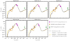 |
Fig. A.1. SEDs for the SCUBA-2 sources with robust AllWISE counterparts. The data-points (see Table A.1) are from AllWISE source catalog (Wright et al. 2010; orange), our SCUBA-2 observations (magenta), and the FIRST survey (Becker et al. 1994; green). We show the SED of M 82 (Silva et al. 1998; black line), of the average ALESS SMG (dashed brown line), and the average ALESS SMG with AV < 1, and AV ≥ 3 (da Cunha et al. 2015; yellow), best fitting only our SCUBA-2 data assuming z = 2.32. |
All Tables
Overdensity estimates at 850 μm from the fit to our true differential number counts with literature functions for blank fields.
All Figures
|
Fig. 1. Galaxy overdensity BOSS1441 at z = 2.32 ± 0.02 (Cai et al. 2017a). The density contours (green) for LAEs are shown in steps of 0.1 galaxies per arcmin2, with the inner density peak of 1.0 per arcmin2. The density contours are shown with increasing thickness for increasing galaxy number density. The brown crosses indicate the positions of known QSOs in the redshift range 2.30 ≤ z < 2.34, and thus likely within the overdensity. We also highlight the position of the ELAN MAMMOTH-1 (dotted crosshair), and the effective area of our SCUBA-2 observations (red dashed contour). |
| In the text | |
|
Fig. 2. SCUBA-2 S/N maps at 850 μm (top panel) and 450 μm (bottom panel) for the field around the ELAN MAMMOTH-1 (red star). The maps are shown with a linear scale from −4 to 4. The size of both maps is 15′ × 15′. Orange circles are the 27 850 μm detections given in Table 2, and yellow squares are the 14 450 μm detections given in Table 3. For both fields, we indicate the noise contours (black dashed) for levels 1.5, 2, and 3× the central noise (σCN; Table 1). The sizes of the circles and squares correspond to 2× the beam FWHM of their respective wavelength. |
| In the text | |
|
Fig. 3. Top: completeness at 850 μm versus flux for different portions of the map, that is, 2σCN < σ < 3σCN, 1.5σCN < σ < 2σCN, σ < 1.5σCN, and < 3σCN (see Fig. 2). Bottom: same as above, but for the 450 μm dataset. |
| In the text | |
|
Fig. 4. Normalized histograms of the S/N values for the pixels within the portions of the 850 and 450 μm maps characterized by less than three times the central noise. The orange and blue histograms indicate the distributions of the jackknife maps, and of the data, respectively. The jackknife maps represents the pixel noise distributions that dominates at low S/N (see Sect. 3.1 for details). The data (especially at 850 μm) shows excesses at high S/N where sources contribute to the distributions. The matched filter technique introduces residual troughs around bright detections, which are visible here as negative excesses. |
| In the text | |
|
Fig. 5. Pure source differential number counts (black data-point) at 850 and 450 μm around the ELAN MAMMOTH-1 compared to the simulated mean counts (red dashed line). The yellow shadings represent the 90% confidence range obtained from 500 realizations of the blue dot-dashed curves. The blue dot-dashed curves are the final adopted underlying models for the Monte Carlo simulations (see Sect. 4), and represent the true number counts. The dashed vertical lines indicate the mean 4σ within the effective area. The horizontal errorbars for the data-points indicate the width of each flux bin. |
| In the text | |
|
Fig. 6. Ratio between the fluxes of the detected sources and the injected sources from the 500 realizations of the estimated underlying counts models (Sect. 4) as a function of the S/N of the detections. The gray dots are ∼100 000 simulated data-points. We show the mean (red) and median (yellow) values of the flux ratio in different S/N bins. The blue dashed curves enclose the 1σ range relative to the mean curve. The test is shown for both 850 (top) and 450 μm (bottom). |
| In the text | |
|
Fig. 7. Positional offset between the detected sources and the injected sources from the 500 realizations of the estimated underlying counts models (Sect. 4) as a function of the S/N of the detections. The gray dots are ∼100 000 simulated data-points. We show the mean (red) and median (yellow) values of the positional offsets in different S/N bins. The blue dashed curves enclose the 1σ range relative to the mean curve. The test is shown for both 850 (top) and 450 μm (bottom). The dot-dashed black lines indicate the predictions from Ivison et al. (2007) based on the LESS sample. |
| In the text | |
|
Fig. 8. Comparison of the SCUBA-2 MAMMOTH-1 differential number counts at 850 μm (top left) and 450 μm (top right), and the cumulative number counts at 850 μm (bottom left) and 450 μm (bottom right) with respect to estimates for blank fields in the literature (Chen et al. 2013b; Casey et al. 2013; Geach et al. 2013, 2017; Wang et al. 2017; Zavala et al. 2017). The black filled symbols are the corrected counts following our Monte Carlo simulations (see Sect. 4), and the blue dot-dashed curves are our true number counts curves from Table 4. When comparing to blank fields, our data for the MAMMOTH-1 field thus show higher counts at 850 μm, but not at 450 μm. |
| In the text | |
|
Fig. 9. Top: fit of the SCUBA-2 MAMMOTH-1 true differential number counts at 850 μm using the functions given in literature works for blank fields (Chen et al. 2013b; Casey et al. 2013; Zavala et al. 2017; Geach et al. 2017) with N0 free to vary. Bottom: SCUBA-2 MAMMOTH-1 true cumulative number counts at 850 μm compared to the fit models obtained in the top panel. In both panels, the blue dot-dashed curve is our true number counts curve from Table 4. All the literature models need a significant increase of their normalization parameter N0 to fit our data at 850 μm, revealing that the covered effective area is overdense with respect to blank fields. We list the values in Table 6. |
| In the text | |
|
Fig. 10. Comparison of the location of the known LAEs within the galaxy overdensity BOSS1441 and the SCUBA-2 submillimeter detections in our field of view (red; as in Fig. 1). We indicate the position of the LAEs (black circles), QSOs in the redshift range 2.30 ≤ z < 2.34 (brown crosses), detections at 850 μm (blue circles; the number indicates the observed flux in unit of mJy; the size of circles equals the FWHM), and detection at 450 μm (yellow squares; the size of symbol equals the FWHM). As in Fig. 1 we show the density contours (green) for LAEs in steps of 0.1 galaxies per arcmin2, with the inner density peak of 1.0 per arcmin2. We also highlight the position of the ELAN MAMMOTH-1 (dotted crosshair), and the field of view of our SCUBA-2 observations for 3× the central noise (red dashed contour). Overall, the LAEs and submillimeter sources are not associated. Only the ELAN MAMMOTH-1 and an additional LAE can be considered as counterparts of a submillimeter detection, MAM-850.14 and MAM-850.16 respectively (highlighted as orange diamonds). Intriguingly the brightest submillimeter detections coincide with the peak of the BOSS1441 overdensity. |
| In the text | |
|
Fig. 11. SED for the source powering the ELAN MAMMOTH-1 at z = 2.319 (source B in Cai et al. 2017b). The data-points are from LBT/LBC imaging and UKIRT/WIRCAM (Cai et al. 2017b and Xu et al. in prep.; blue), AllWISE source catalog (Wright et al. 2010; orange), our SCUBA-2 observations (magenta), and the FIRST survey (Becker et al. 1994; green). Left panel: data-points in comparison to the SED of M 82 (Silva et al. 1998; black line), of the average ALESS SMGs (dashed brown line), and of the average ALESS SMGs with AV < 1 (da Cunha et al. 2015; yellow), best fitting our data-points for z = 2.319. The best agreement is found for the M82 template, but the W3 data-point is underestimated. Right panel: data-points in comparison to the best fit of AGNfitter (gray line), together with the individual components: hot dust emission (purple), cold dust emission (green), stellar emission (yellow), and the emission from the accretion disk (blue). The hot dust contribution allows a better fit to the data. |
| In the text | |
|
Fig. A.1. SEDs for the SCUBA-2 sources with robust AllWISE counterparts. The data-points (see Table A.1) are from AllWISE source catalog (Wright et al. 2010; orange), our SCUBA-2 observations (magenta), and the FIRST survey (Becker et al. 1994; green). We show the SED of M 82 (Silva et al. 1998; black line), of the average ALESS SMG (dashed brown line), and the average ALESS SMG with AV < 1, and AV ≥ 3 (da Cunha et al. 2015; yellow), best fitting only our SCUBA-2 data assuming z = 2.32. |
| In the text | |
Current usage metrics show cumulative count of Article Views (full-text article views including HTML views, PDF and ePub downloads, according to the available data) and Abstracts Views on Vision4Press platform.
Data correspond to usage on the plateform after 2015. The current usage metrics is available 48-96 hours after online publication and is updated daily on week days.
Initial download of the metrics may take a while.