Molecular gas in radio galaxies in dense megaparsec-scale environments at z = 0.4–2.6

G. Castignani; F. Combes; P. Salomé; C. Benoist; M. Chiaberge; J. Freundlich; G. De Zotti

doi:10.1051/0004-6361/201834066

Home

All issues

Volume 623 (March 2019)

A&A, 623 (2019) A48

Full HTML

Free Access

Issue		A&A Volume 623, March 2019


Article Number		A48
Number of page(s)		23
Section		Cosmology (including clusters of galaxies)
DOI		https://doi.org/10.1051/0004-6361/201834066
Published online		04 March 2019

A&A 623, A48 (2019)

Molecular gas in radio galaxies in dense megaparsec-scale environments at z = 0.4–2.6

G. Castignani¹^,2^,3, F. Combes²^,3, P. Salomé², C. Benoist⁴, M. Chiaberge⁵^,6, J. Freundlich⁷ and G. De Zotti⁸

¹ Laboratoire d’Astrophysique, École Polytechnique Fédérale de Lausanne (EPFL), Observatoire de Sauverny, 1290 Versoix, Switzerland
e-mail: gianluca.castignani@epfl.ch
² Sorbonne Université, Observatoire de Paris, Université PSL, CNRS, LERMA, 75014 Paris, France
³ Collège de France, 11 Place Marcelin Berthelot, 75231 Paris, France
⁴ Université Côte d’Azur, Observatoire de la Côte d’Azur, CNRS, Laboratoire Lagrange, Blvd de l’Observatoire, CS 34229, 06304 Nice Cedex 4, France
⁵ Space Telescope Science Institute, 3700 San Martin Dr., Baltimore, MD 21210, USA
⁶ Johns Hopkins University, 3400 N. Charles Street, Baltimore, MD 21218, USA
⁷ Centre for Astrophysics and Planetary Science, Racah Institute of Physics, The Hebrew University, Jerusalem 91904, Israel
⁸ INAF-Osservatorio Astronomico di Padova, Vicolo dell’Osservatorio 5, 35122 Padova, Italy

Received: 10 August 2018
Accepted: 24 December 2018

Abstract

Context. Low luminosity radio galaxies (LLRGs) typically reside in dense megaparsec-scale environments and are often associated with brightest cluster galaxies (BCGs). They are an excellent tool to study the evolution of molecular gas reservoirs in giant ellipticals, even close to the active galactic nucleus.

Aims. We investigate the role of dense megaparsec-scale environment in processing molecular gas in LLRGs in the cores of galaxy (proto-)clusters. To this aim we selected within the COSMOS and DES surveys a sample of five LLRGs at z = 0.4−2.6 that show evidence of ongoing star formation on the basis of their far-infrared (FIR) emission.

Methods. We assembled and modeled the FIR-to-UV spectral energy distributions (SEDs) of the five radio sources to characterize their host galaxies in terms of stellar mass and star formation rate. We observed the LLRGs with the IRAM-30 m telescope to search for CO emission. We then searched for dense megaparsec-scale overdensities associated with the LLRGs using photometric redshifts of galaxies and the Poisson Probability Method, which we have upgraded using an approach based on the wavelet-transform (wPPM), to ultimately characterize the overdensity in the projected space and estimate the radio galaxy miscentering. Color-color and color-magnitude plots were then derived for the fiducial cluster members, selected using photometric redshifts.

Results. Our IRAM-30 m observations yielded upper limits to the CO emission of the LLRGs, at z = 0.39, 0.61, 0.91, 0.97, and 2.6. For the most distant radio source, COSMOS-FRI 70 at z = 2.6, a hint of CO(7→6) emission is found at 2.2σ. The upper limits found for the molecular gas content M(H₂)/M_⋆ < 0.11, 0.09, 1.8, 1.5, and 0.29, respectively, and depletion time τ_dep ≲ (0.2−7) Gyr of the five LLRGs are overall consistent with the corresponding values of main sequence field galaxies. Our SED modeling implies large stellar-mass estimates in the range log(M_⋆/M_⊙) = 10.9−11.5, typical for giant ellipticals. Both our wPPM analysis and the cross-matching of the LLRGs with existing cluster/group catalogs suggest that the megaparsec-scale overdensities around our LLRGs are rich (≲10¹⁴ M_⊙) groups and show a complex morphology. The color-color and color-magnitude plots suggest that the LLRGs are consistent with being star forming and on the high-luminosity tail of the red sequence. The present study thus increases the still limited statistics of distant cluster core galaxies with CO observations.

Conclusions. The radio galaxies of this work are excellent targets for ALMA as well as next-generation telescopes such as the James Webb Space Telescope.

Key words: galaxies: active / galaxies: clusters: general / galaxies: star formation / molecular data

© ESO 2019

1. Introduction

Radio galaxies are powerful extra-galactic sources with low-frequency radio luminosities in the range ∼10⁴¹⁻⁴⁶ erg s⁻¹. They are typically hosted by giant ellipticals and associated with the most massive ≳10⁸ M_⊙ black holes. The majority of the radio galaxies, at least in the local universe, have little molecular gas to feed star formation and the central nuclear regions (Lim et al. 2000, 2004; Evans et al. 2005; Ocaña Flaquer et al. 2010; Baldi et al. 2015).

However in the distant universe (z ≳ 2) large reservoirs of ≳10¹⁰ M_⊙ of molecular gas have commonly been found in powerful high-z radio galaxies (Scoville et al. 1997; Alloin et al. 2000; Papadopoulos et al. 2000; De Breuck et al. 2003a,b, 2005; Greve et al. 2004; Klamer et al. 2005; Ivison et al. 2008, 2011; Nesvadba et al. 2009; Emonts et al. 2011). We refer to Miley & De Breuck (2008) for a review.

Low luminosity radio galaxies (LLRGs) with low-radio frequency luminosities ≲5 × 10⁴¹ erg s⁻¹ at 178 MHz represent the great majority among the radio galaxy population, because of the steepness of the radio luminosity function. However, mainly because of their intrinsically low radio power, LLRGs are difficult to find in the distant universe (Snellen & Best 2001; Chiaberge et al. 2009; Mauch & Sadler 2007; Donoso et al. 2009; Smolčić et al. 2009).

Remarkably, LLRGs are often hosted by giant ellipticals of cD type (Zirbel 1996), which are typically associated with the brightest cluster galaxies (BCGs, von der Linden et al. 2007; Yu et al. 2018). The vast majority (∼70%) of LLRGs are in fact found in rich groups and clusters, out to z ∼ 2, almost independently of the redshift (Hill & Lilly 1991; Zirbel 1997; Wing 2011; Castignani et al. 2014a,b; Paterno-Mahler et al. 2017). LLRGs are therefore a precious tool to search for distant galaxy groups and clusters as well as BCGs.

The BCGs are unique laboratories to study the effect of dense galaxy cluster environment on galaxy evolution. They are located at the center of the cluster cores (Lauer et al. 2014) and exhibit exceptional masses and luminosities. They are believed to evolve via phenomena such as dynamical friction (White 1976), galactic cannibalism (Hausman & Ostriker 1978), interactions with the intracluster medium (Stott et al. 2012), and cooling flows (Salomé et al. 2006). In the local universe some studies have shown evidence of molecular gas reservoirs in BCGs (Edge 2001; Salomé & Combes 2003; Hamer et al. 2012; McNamara & Russell 2014; Russell et al. 2014; Tremblay et al. 2016), however little is known about the evolution of such reservoirs and the formation of BCGs.

Recent work suggests that BCGs have doubled their stellar mass since z ∼ 1 (Lidman et al. 2012), which is consistent with a global picture where BCGs evolve via dry accretion of satellite galaxies (Collins et al. 2009; Stott et al. 2011). More recent studies have however found potentially conflicting results to this somewhat simplistic hypothesis. Possible evidence for high levels of star formation and large reservoirs of molecular gas has in fact been suggested for BCGs and cluster core galaxies out to z ∼ 1 and beyond (Brodwin et al. 2013; Zeimann et al. 2013; Webb et al. 2013, Webb et al. 2015a,b; Alberts et al. 2016; McDonald et al. 2016; Bonaventura et al. 2017), possibly privileging the late assembly of cluster core members via both strong environmental quenching mechanisms (e.g., strangulation, ram pressure stripping, and galaxy harassment; Larson et al. 1980; Moore et al. 1999) and rapid infall of gas feeding star formation at high-z (reaching a maximum at z ∼ 2−3), followed by slow cooling flows at low-z (Ocvirk et al. 2008; Dekel et al. 2009a,b).

In this work we study the molecular gas properties of a sample of five star forming LLRGs at z = 0.4−2.6 that have been selected since they show evidence of significant star formation based on their far-infrared (FIR) emission. With the present work we aim to i) probe the molecular gas content and ii) investigate the role of dense megaparsec-scale environment in processing molecular gas of distant LLRGs in the cores of galaxy (proto-)clusters. The five radio sources are in fact hosted in dense megaparsec-scale environments and are potentially the high-z progenitors of present day star forming (>40 M_⊙/yr) local BCGs such as the famous Perseus A and Cygnus A (Fraser-McKelvie 2014).

This work is the second reporting the results of a wider search for molecular gas in distant cluster galaxies (see also Castignani et al. 2018). The paper is structured as follows. In Sect. 2 we introduce the LLRG sample; in Sect. 3 we report our IRAM-30 m observations and data reduction; in Sect. 4 we describe the wavelet-based Poisson Probability Method, which we developed and applied to search for distant (proto-)clusters around LLRGs; in Sect. 5 we present our results; in Sect. 6 we discuss the results; and in Sect. 7 we draw our conclusions.

In this study we refer to megaparsec-scale overdensities, galaxy clusters, galaxy groups, and proto-clusters, with no specific distinction. However we stress that the megaparsec-scale overdensities associated with the LLRGs in our sample may have different properties. In particular they may be still forming proto-clusters, virialized clusters, or lower-mass groups (see e.g., Overzier 2018, for a review).

Throughout this work we adopt a flat ΛCDM cosmology with matter density Ω_m = 0.30, dark energy density Ω_Λ = 0.70, and Hubble constant h = H₀/100 km s⁻¹ Mpc⁻¹ = 0.70 (see however, Planck Collaboration VI 2018; Riess et al. 2016, 2018).

2. The radio galaxy sample

The Dark Energy Survey (DES, The Dark Energy Survey Collaboration 2005, 2016) is an ongoing five-year project (2013–2018) composed of two distinct multi-band imaging surveys: a ∼5000 deg² wide-area grizY survey and a deep supernova griz survey made by six distinct deep fields (Kessler et al. 2015). The coadded source catalog and images from the first 3 yr of science operations have recently been made public as part of the first public data release (DES DR1, Abbott et al. 2018)¹.

The Very Large Array Faint Images of the Radio Sky at Twenty-centimeters (VLA FIRST) survey (Becker et al. 1995) observed 10 000 deg² of the North and South Galactic Caps at 1.4 GHz. Post-pipeline radio maps have a typical full width at the half maximum (FWHM) resolution of ∼5 arcsec. The detection limit of the FIRST source catalog is ∼1 mJy with a typical rms of 0.15 mJy.

In order to select the radio galaxy sample we have limited ourselves to the DES supernova (SN) deep fields that overlap with the FIRST survey. This selection yielded four fields, namely the DES SN deep fields numbered 2, 3, 5, and 6. Field number 6 is located at approximately (RA; Dec) = (209.5; 4.9) deg and covers ∼4 deg². It is not included in the DES DR1 survey area, and is therefore not considered in this work. Fields 2 and 3 are located at approximately (RA; Dec) = (35.5; −5.5) deg and (42.0; −0.4) deg, and subtend ∼16 deg² and ∼10 deg² of solid angle in the sky, respectively. They are both included in the DES DR1 and are therefore considered in this work. Field number 5 is located at approximately (RA; Dec) = (150.0; 2.2) deg and covers ∼4 deg². It is not included in the DES DR1, but it entirely includes the 2 deg² Cosmic Evolution Survey (COSMOS, Scoville et al. 2007) that is considered in this work. Concerning the sample selection and characterization in the following we separately consider the DES SN deep fields 2 and 3 (Sect. 2.1), and the COSMOS survey (Sect. 2.2).

With the present work we aim at studying the molecular gas properties of a pilot sample of rare distant BCG candidates with suggested evidence of ongoing star formation. For this pilot study we considered the DES SN deep fields because they partially overlap with the VLA FIRST survey and because their deep observations (down to AB magnitudes ∼24.5 in all DES bands) enable us to effectively find and characterize both distant LLRGs and their megaparsec-scale environments.

2.1. DES radio galaxies 399 and 708

We aim at selecting radio galaxies to be followed-up with radio facilities at millimeter (mm) wavelengths. Accurate redshift measurements are therefore needed: they have to be used as a positional prior for the follow-ups. We consider DES DR1 sources in the DES SN deep fields 2 and 3 and search for their spectroscopic redshifts from both the Fourteenth Data Release² (DR14) of the Sloan Digital Sky Survey (SDSS) and the DES spectroscopic dataset (C. Benoist, priv. comm.). Since the astrometric precision of SDSS and DES is ≃0.1 arcsec we adopted a search radius of 1 arcsec. This selection yielded 33 148 unique spectroscopic counterparts. We aim at studying distant radio galaxies. We therefore limit ourselves to galaxies with spectroscopic redshifts z > 0.3. This selection yielded 22 778 spectroscopic sources.

We have adopted the DES magnitudes corrected for Galactic extinction, as listed in the DES DR1 coadd catalog (DR1_MAIN) and denoted, for example, MAG_AUTO_G_DERED (we refer to Appendix D of Abbott et al. 2018, for further details).

2.1.1. FIRST

We searched for radio counterparts of the DES sources using the FIRST source catalog and a search radius of 3 arcsec, consistently with the positional accuracy ∼1 arcsec of FIRST sources. The search yielded 151 unique low-frequency radio counterparts.

2.1.2. WISE

One of the main goals of this work is to select a sample of star forming radio galaxies. We have therefore selected a sub-sample of radio sources with 22 μm emission in the observer frame, as found by the W4 filter of the Wide-field Infrared Survey Explorer (WISE, Wright et al. 2010). We have cross-correlated our DES sources with the allWISE source catalog³ by adopting a search radius of 6.5 arcsec, consistently with previous studies on distant radio sources (e.g., Castignani et al. 2013). The search yielded 50 sources with unique WISE counterparts and W4 magnitudes with signal-to-noise ratio S/N > 1. A detailed study of such a sample will be performed in a forthcoming paper (Castignani et al., in prep.).

Among the 50 sources we have selected two galaxies that we observed with the IRAM-30 m telescope, as part of a pilot project to search for CO in distant star-forming galaxies. The two selected galaxies are both within the DES SN deep field number 3 and are denoted hereafter as DES-RG 399 and 708, where RG stands for radio galaxy. They have WISE counterparts in the allWISE source catalog with W4 magnitudes reported at 2.1σ and 1.5σ, respectively. In the other WISE W1, W2, and W3 channels the sources are detected at S/N > 9.5, with the exception of DES-RG 708 whose WISE W3 emission at 12 μm in the observer frame is found at 2.5σ.

The two galaxies have spectroscopic redshifts z = 0.39 and 0.61, respectively. In order to characterize the broad band emission of both sources we searched for additional data using the DES coordinates as input, as described in the following.

2.1.3. NVSS

The NRAO VLA Sky Survey (NVSS) survey (Condon et al. 1998) at 1.4 GHz was obtained using the VLA-D configuration. The FWHM angular resolution of the NVSS radio maps is 45 arcsec. Therefore, NVSS is more suitable than FIRST for detecting extended emission. We found NVSS counterparts for both DES-RG 399 and 708, at an angular separation of 1.2 arcsec and 2.4 arcsec, respectively. Their NVSS fluxes are (12.0 ± 0.6) mJy and (36.0 ± 1.5) mJy, respectively, while the FIRST fluxes are 12.54 mJy and 11.80 mJy. An additional southern source is detected by FIRST at an angular separation of ∼7.2 arcsec from DES-RG 708 with a flux of 12.63 mJy; it is visible in the VLA-FIRST image (Fig. 1, top). DES-RG 708 might have an extended radio morphology, unresolved by NVSS. Alternatively, it is also possible that the radio source has a radio morphology with two hot-spots, typical of FR II radio sources (Fanaroff & Riley 1974). The available angular resolution does not allow us to distinguish between the two scenarios.

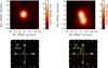Fig. 1.

VLA FIRST (top panel) and composite SDSS DR14 (bottom panel) images centered at the DES coordinates of DES-RG 399 (left panel) and DES-RG 708 (right panel). All images have 30″ × 30″ sizes and north is up, east is left.

2.1.4. IRAS

We searched for FIR counterparts of our sources within the Infrared Astronomical Satellite (IRAS) Faint Source Catalog (Moshir et al. 1990) and the IRAS Point Source Catalog (Helou & Walker 1988). Neither of the two DES-RGs was found. We extracted 15′ × 15′ IRAS Sky Survey Atlas (ISSA) image cutouts⁴ at 12, 25, 60, and 100 μm, centered at the coordinates of our DES-RG sources. The pixel size of the images is 90 arcsec that corresponds to ∼(500–600) kpc for DES-RG 399 and 708, which are therefore unresolved. We then estimated 3σ upper limits to the IRAS fluxes as three times the rms dispersion derived from the cutout images of the two sources.

2.1.5. UKIDSS

The UKIRT Infrared Deep Sky Survey (UKIDSS) mapped the near-infrared (NIR) sky (Lawrence et al. 2007). UKIDSS used the UKIRT Wide Field Camera (WFCAM, Casali et al. 2007). The photometric system is described in Hewett et al. (2006), and the calibration is described in Hodgkin et al. (2009). The pipeline processing and science archive are described in Hambly et al. (2008). The UKIDSS Large Area Survey (LAS)⁵ consists of observations covering 7500 deg² of the sky at the YJHK NIR bands and includes the DES SN deep field number 3. We searched within the latest public release UKIDSSDR10PLUS and found unique UKIDSS counterparts for both DES sources using a search radius of 3 arcsec, which is consistent with the positional FWHM accuracy ≲1.2 arcsec of UKIDSS (Lawrence et al. 2007). The two counterparts are located at angular separations of 0.5 arcsec and 0.2 arcsec from the DES coordinates of DES-RG 399 and 708, respectively. UKIDSS Vega magnitudes, derived within a 2 arcsec aperture, were converted into the AB system by applying the offsets reported in Table 7 of Hewett et al. (2006). The magnitudes were also corrected for Galactic extinction using the extinction curve by Cardelli et al. (1989), as updated by O’Donnell (1994) and normalized to A(V) = 3.1E(B − V). For each source, the value of E(B − V) was estimated using the extinction values reported for the SDSS bands and the prescriptions described in SDSS DR14 tutorial⁶.

2.1.6. SDSS

The DES SN deep field number 3 is entirely contained within the SDSS survey area. We found unique SDSS DR14 optical counterparts at the u, g, r, i, and z bands of SDSS for both sources using a search radius of 1 arcsec. We adopted the SDSS magnitudes corrected for Galactic extinction, as listed in the DR14 catalog and denoted, for example, dered_g. As suggested in the DR14 tutorial⁷ we decreased the DR14 u-band magnitudes by 0.04 to convert them into the AB system. For the other bands the corrections are negligible. In Fig. 1 (bottom) we show the SDSS images of DES-RG 399 and 708.

2.1.7. GALEX

We searched for UV photometry of our DES radio sources in the joint sixth and seventh data releases, GR 6/7⁸, of the Galaxy Evolution Explorer (GALEX) satellite (Morrissey et al. 2007). GALEX provides near-ultraviolet (NUV, 1750–2800 Å) and far-UV (FUV, 1350–1750 Å) source fluxes down to a magnitude limit AB ∼ 20–21 with an estimated positional accuracy of ∼0.5 arcsec. By adopting a search radius of 2 arcsec we found a possible GALEX counterpart for one of the two sources, namely DES-RG 399, at an angular separation of 1.8 arcsec. However DES-RG 399 has a companion located at 1.8 arcsec of angular separation, visible in the SDSS image (see Fig. 1). The GALEX source is located at an angular separation of 1.3 arcsec from this companion and it is therefore possible that it is not associated with the source DES-RG 399. Visual inspection of the IR-to-UV spectral energy distribution (SED) of DES-RG 399 further strengthens such a possibility. We therefore preferred to remove the GALEX association for DES-RG 399.

In Table 1 we summarize the IR-to-optical photometric data of the two DES-RG sources. We note that DES and SDSS magnitudes of the two DES-RG sources are discrepant up to ∼0.7 mag. DES-RG 399 and 708 are primarily selected at low radio frequency (FIRST) by adopting a search radius of 1 arcsec that is used to look for the optical DES counterparts. This radio positional uncertainty implies that we cannot completely rule out the possibility that the discrepancy in the magnitudes is due to the companions of the radio sources, which are in fact visible in the optical images at angular separations of the order of ∼1 arcsec (see Fig. 1, bottom).

Table 1.

Photometry of DES-RG 399 and 708.

2.2. COSMOS-FRI radio galaxies 16, 31, and 70

2.2.1. Target selection

COSMOS is a multiwavelength equatorial 2 deg² survey (Scoville et al. 2007) that includes Hubble Space Telescope (HST) observations (Koekemoer et al. 2007) and IR Spitzer imaging (S-COSMOS, Sanders et al. 2007). We limit ourselves to the sample of well-studied distant z ∼ 1−3 FR I (Fanaroff & Riley 1974) radio galaxy candidates described in Chiaberge et al. (2009) and further reconsidered on the basis of their radio power by Castignani et al. (2014a).

With the aim of selecting a sample of distant radio galaxies to be followed-up with radio facilities at mm wavelengths we restrict ourselves to the subsample of COSMOS-FRIs with available spectroscopic redshifts (see Baldi et al. 2013; Castignani et al. 2014a, for further details), similarly to what was done in Sect. 2.1. This selection yielded eight sources, namely, COSMOS-FRI 1, 16, 27, 66, 31, 52, 70, and 258. A ninth source, 236, is included in the Chiaberge et al. (2009) sample and has a spectroscopic redshift. However it is excluded from our analysis because it is a confirmed QSO at z = 2.132 (Prescott et al. 2006). The source COSMOS-FRI 70 has no spectroscopic redshift from the literature. However we verified (M. Bolzonella, priv. comm.) that it is the only COSMOS-FRI with a spectroscopic counterpart within the zCOSMOS-deep catalog (Lilly et al. 2007, Lilly et al., in prep.)⁹, which includes approximately 10 000 galaxies of the COSMOS survey at approximately 1.5 < z < 3.0. We therefore included COSMOS-FRI 70 in our analysis.

Baldi et al. (2013), hereafter B13, carefully reconsidered the IR, optical, and UV photometric data associated with the COSMOS-FRIs of the Chiaberge et al. (2009) sample and performed SED fits to the data. On the other hand the associations provided in the COSMOS photometric catalogs are performed automatically (e.g., Ilbert et al. 2009; Laigle et al. 2016). Therefore in this work we adopt the photometric data provided in B13 for the COSMOS-FRI galaxies. In particular, since we aim to select star forming galaxies we restrict ourselves to the subsample of sources with available Spitzer MIPS flux at 23.68 μm from B13. This selection yielded three sources, namely COSMOS-FRI 16, 52, and 70. We also included COSMOS-FRI 31 because it has a WISE counterpart with W4 magnitude reported at 0.9σ in the allWISE source catalog, while we discarded COSMOS-FRI 52 because we verified that its redshifted CO lines cannot be optimally observed. Therefore we limit our analysis to COSMOS-FRI 16, 31, 70. In Fig. 2 we report the radio and optical images of the three COSMOS-FRI sources considered.

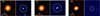Fig. 2.

Radio and optical images from Chiaberge et al. (2009) for the COSMOS-FRI sources in our sample. For each source, the image in the left panel is from the VLA-COSMOS survey (Schinnerer et al. 2007), while in the right panel the HST-COSMOS ACS image (F814W) is shown (Koekemoer et al. 2007).

2.2.2. Infrared-to-ultraviolet photometric data

For the three COSMOS sources the IR-to-optical photometry reported by B13 and considered in this work includes data from the Canada-France-Hawaii Telescope (CFHT, Boulade et al. 2003), UKIRT (Casali et al. 2007), NOAO (Capak et al. 2007), Subaru (Taniguchi et al. 2007), Spitzer IRAC and Spitzer MIPS at 23.68 μm (Sanders et al. 2007), HST (Koekemoer et al. 2007), and GALEX (Morrissey et al. 2007). We also included 3σ upper limits for the Spitzer MIPS fluxes at 70 μm and 160 μm, corresponding to 5.1 mJy and 39 mJy, respectively (Lee et al. 2010).

Following a procedure similar to that described in Sect. 2.1.2, WISE counterparts were found for all three sources except COSMOS-FRI 70. Similarly, COSMOS-FRI 31 is not detected in the WISE W3 channel. Analogously to previous work by Castignani & De Zotti (2015), in these cases, where WISE fluxes are absent, we have adopted 3σ flux density upper limits of 0.6 and 3.6 mJy, due to instrumental noise alone (Wright et al. 2010), for the WISE channels W3 and W4, respectively. For channels W1 and W2 the 3σ limits are set by confusion noise and are equal to 0.31 and 0.17 mJy, respectively (Jarrett et al. 2011). COSMOS-FRI 31, in the W4 channel, and COSMOS-FRI 16, in both W3 and W4 channels, are only marginally detected by WISE, at S/N < 2. We therefore converted the associated fluxes into 3σ upper limits. In Table 2 we summarize the IR-to-UV photometry of COSMOS-FRI 16, 31, and 70.

Table 2.

Photometry of COSMOS-FRI 16, 31, and 70.

The NIR-to-optical magnitudes of these three COSMOS-FRI sources were then corrected for Galactic extinction by adopting a procedure analogous to that described in Sect. 2.1.5. For each source the value of E(B − V) was obtained assuming the value for Galactic extinction estimated by Schlafly & Finkbeiner (2011) at the source location and normalized to A(V) = 3.1E(B − V).

Our final sample comprises five sources, DES-RG 399, DES-RG 708, COSMOS-FRI 16, COSMOS-FRI 31, and COSMOS-FRI 70. In the following we describe the SED modeling for these sources.

2.3. SED modeling

We assembled the IR-to-UV SEDs for the five sources in our sample using the photometric dataset described above and performed fits to the SEDs using LePhare (Arnouts et al. 1999; Ilbert et al. 2006). Following the prescriptions provided for the LePhare code, we fitted the FIR data separately to account for possible dust emission, using the Chary & Elbaz (2001) library consisting of 105 templates. The remaining photometric points at shorter wavelengths were fitted using the CE_NEW_MOD library provided by LePhare, which is similar to that described in Arnouts et al. (1999) and consists of 66 templates based on linear interpolation of the four original SEDs of Coleman et al. (1980). The SEDs along with their best fits are reported in Fig. 3 for all five sources in our sample.

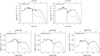Fig. 3.

SEDs and modeling for DES-RG (top panel) and COSMOS-FRI (bottom panel) sources in the sample. Data-points for DES-RG sources are from SDSS (red pentagons), DES (blue squares), UKIDSS (black stars), WISE (green triangles), and IRAS (yellow upper limits), while those for COSMOS-FRI galaxies are archival NIR-to-UV data from B13 (blue open diamonds). Spitzer-IRAC (open black dots), Spitzer-MIPS (pink open crosses and upper limits), and WISE (green open triangles and upper limits) data are also included for COSMOS-FRI galaxies. See text for further details. Dashed and solid lines show the best fit models for the stellar and dust components, respectively.

We stress that B13 already reported the IR-to-UV SED modeling for the COSMOS-FRI sources considered in this work. However we preferred to perform the SED fitting independently because we want to report homogeneous results for all galaxies considered in this work, including the DES-RG sources not considered by B13. Furthermore, B13 did not include Spitzer MIPS upper limits at 70 and 160 μm and did not provide SFR estimates; see also the following sections.

2.4. Radio luminosities

In this section we estimate the radio luminosities for the five radio sources in our sample. Similarly to previous work (Chiaberge et al. 2009; Castignani et al. 2014a) we assume that the radio spectrum in the region around the frequency 1.4 GHz is a power-law of the form S_ν ∝ ν^−α, where S_ν is the radio flux density at the observer frequency ν and the spectral index α is assumed to be α = 0.8. We adopt the NVSS flux densities reported in Sect. 2.1.3 for DES-RG 399 and 708, while those of COSMOS-FRI 16, 31, and 70 are taken from Castignani et al. (2014a). We then estimate the rest frame 1.4 GHz luminosity density as follows:

$\begin{matrix} L_{1.4 GHz} = 4 π S_{1.4 GHz} D_{L} {(z)}^{2} {(1 + z)}^{α - 1}, \end{matrix}$ $\begin{aligned} L_{1.4\,\mathrm{GHz}} = 4\pi S_{1.4\,\mathrm{GHz}}D_{\rm L}(z)^2\left(1+z\right)^{\alpha -1}, \end{aligned}$ (1)

where S_1.4 GHz is the observed 1.4 GHz flux density, D_L is the luminosity distance, and α is the radio spectral index. Low-radio frequency and additional properties for all five sources in our sample are summarized in Table 3.

Table 3.

Properties of our targets.

The radio power of our sources is fairly consistent with that of low-luminosity FR I radio galaxies belonging to the FR I class¹⁰, for which L_1.4 GHz ≲ 2.6 × 10³² erg s⁻¹ Hz⁻¹. From the values reported in Table 3 we observe that only DES-RG 708 and COSMOS-FRI 70 have values of L_1.4 GHz that are higher than the reported FR I/FR II radio-power divide. However we stress that their radio luminosities are still fairly consistent with the high-power tail of FR I radio galaxies, since they are at least one order of magnitude less bright than powerful distant radio galaxies at similar redshifts (Miley & De Breuck 2008; Ineson et al. 2013). We refer to Castignani et al. (2014a) for further discussion about the radio power properties of the COSMOS-FRI sources.

In the following we describe our IRAM-30 m observations and data analysis.

3. IRAM-30 m observations and data reduction

We observed the five radio galaxies in our sample using the IRAM-30 m telescope at Pico Veleta in Spain. The observations of our targets were carried out in the summers of 2016 and 2017 as part of two observational programs (P.I.: Castignani).

We used the Eight Mixer Receiver (EMIR) and its E230 band to observe a CO(J → J–1) emission line from each target source, at frequencies between 215 and 249 GHz, where J is a positive integer denoting the total angular momentum. For each source the specific CO(J → J–1) transition was chosen to maximize the likelihood for the detection in terms of the ratio of the predicted signal to the expected rms noise. We refer to Table 4 for further details.

Table 4.

Molecular gas properties.

In the ∼(1.2–1.4) mm wavelength range, the E230 receiver can offer 4 × 4 GHz instantaneous bandwidth covered by the correlators. Of these four bands (UI, UO, LI, LO), we used only the lower side bands (LI, LO). The wobbler-switching mode was used for all the observations with a frequency of 0.5 Hz and a throw of either 60 arcsec or 120 arcsec, depending on the specific wind conditions found during the observations. The adopted wobbler throw is conservatively higher than the size of our target sources, which is in fact less than a few arcseconds.

The Wideband Line Multiple Autocorrelator (WILMA) was used to cover the LI-4 GHz band in each linear polarization. The WILMA back-end gives a resolution of 2 MHz. We also simultaneously recorded the data with the Fast Fourier Transform Spectrometers (FTS), as a backup, at 200 kHz resolution, to cover the 2 × 4 GHz lower sidebands (LI and LO), for each linear polarization.

The five target sources were observed for an on-source observing time of ∼71 h in total, distributed among the five sources as follows: 6.8 h (DES-RG 399), 17.8 h (DES-RG 708), 14.0 h (COSMOS-FRI 16), 12.4 h (COSMOS-FRI 31), and 20.1 h (COSMOS-FRI 70).

Sources COSMOS-FRI 16 and 31 were observed during August 17–22, 2016, in bad weather conditions. Observations were carried out with an average precipitation water vapor (pwv) value of ∼12 mm, as well as high average system temperatures T_sys = 615 K and 898 K, for COSMOS-FRI 16 and 31, respectively. Sources DES-RG 399, DES-RG 708, and COSMOS-FRI 70 were observed during September 10–12, 2017, in very good weather conditions. Observations were carried out with average pwv values of 2.9 mm, 3.5 mm, and 1.5 mm, as well as average T_sys = 219 K, 327 K, and 294 K, for DES-RG 399, DES-RG 708, and COSMOS-FRI 70, respectively.

Only minor flagging was required: three scans, corresponding to 0.2 h (on-source) of observations, were removed for COSMOS-FRI 31 because of bad weather conditions during their acquisition. The time reported above for COSMOS-FRI 31 corresponds to the net on-source time, where such scans have been removed.

Data reduction and analysis were performed using the CLASS software of the GILDAS package¹¹. The results are reported in Sect. 5.3.

4. The wavelet-based Poisson Probability Method (wPPM)

We searched for megaparsec-scale overdensities around the radio galaxies in our sample using photometric redshifts of galaxies and the Poisson Probability Method (PPM, Castignani et al. 2014a,b), that we have improved using an approach based on the wavelet transform. We denote the upgraded PPM as wPPM, where hereafter w refers to the wavelet transform. In Sect. 4.1 we describe the photometric redshift catalogs used in this work. In Sect. 4.2 we outline the PPM procedure, while in Sect. 4.3 we describe its wavelet-based upgrade. In Sect. 5.5 we describe the wPPM results for the radio sources in our sample.

4.1. Photometric redshift catalogs

We used photometric redshifts provided for the SDSS survey to search for megaparsec-scale overdensities around DES-RG 399 and 708. Photometric redshifts of SDSS DR14 are estimated using a machine learning technique described in Csabai et al. (2007) and named kd-tree nearest-neighbor fit. We retrieved photometric redshifts within a rectangular field delimited by 40.2 deg < RA < 43.8 deg. and −1.8 deg < Dec < 1.0 deg. Such a region corresponds approximately to the DES SN deep field n. 3 survey. Following the SDSS DR14 tutorial¹² we considered sources with photoErrorClass = −1, 1, 2, or 3, which correspond to photometric redshifts with estimated rms errors in the range ≃(0.043−0.074).

Concerning COSMOS-FRI 16, 31, and 70 we used the official COSMOS photometric redshift catalogs (Ilbert et al. 2009; Laigle et al. 2016). These catalogs are both obtained using the large multiwavelength photometric dataset provided for the COSMOS survey, which includes observations from the HST, CFHT, and Subaru. The photometric redshift catalog by Laigle et al. (2016) includes also YJHKs photometry from the UltraVISTA survey (McCracken et al. 2012). Both photometric redshift catalogs were obtained by performing fits to the SEDs using LePhare (Arnouts et al. 1999; Ilbert et al. 2006).

4.2. The PPM procedure

We summarize here the basic steps of the PPM. We refer to Castignani et al. (2014b) for a detailed description.

We tessellate the projected space with a circle centered at the coordinates of the radio galaxy and a number of consecutive adjacent annuli. The annuli and the central circle have equal area of 2.18 arcmin². In particular the circle has a radius of 50 arcsec, which corresponds to physical scales in the range ≃(0.3–0.4) Mpc for the sources in our sample.
For each region of the tessellation (the central circle and the consecutive annuli), we count the number of sources with photometric redshifts within an interval of length Δz and centered at the centroid redshift z_centroid. The parameters Δz and z_centroid uniformly span a grid of values that reflect the photometric redshift uncertainties and correspond to the redshift range of our interest, respectively.
For each pair (z_centroid; Δz) we calculate the probability of the null hypothesis (i.e., no clustering) based on source number counts and Poisson statistics. To this aim the galaxy number density associated with each region of the tessellation is compared to that inferred from a sufficiently large control region. We chose rectangular control regions with subtended areas of 1.96 deg² and 1.44 deg² and with centers coincident to those of DES SN deep field n. 3 and COSMOS, respectively. The control regions are safely contained by the two surveys. The procedure yields a number count excess significance associated with each pair (z_centroid; Δz), as well as a maximum radius within which the overdensity is detected. Namely, the procedure selects the first consecutive regions starting from the central circle for which the probability of the null hypothesis is ≤ 30%, for each pair (z_centroid; Δz).
The PPM plots for the fields of the radio sources are derived. For each pair (z_centroid; Δz) the detection significance defined in the previous step is plotted.
As noted in Castignani et al. (2014a,b) noisy features are present in the PPM plots because of photometric redshift uncertainties and shot noise associated with photometric redshift number counts. These noisy patterns might lead to spurious overdensity-to-radio-galaxy associations, especially in the case where the redshift of the radio galaxy is the photometric one. However, at variance with the original PPM procedure, we decided not to use any Gaussian filter to eliminate high-frequency noisy patterns. This choice was motivated by the fact that we know the spectroscopic redshift of each radio galaxy. Such knowledge minimizes the chance of a spurious association between the radio source and the overdensities detected by the PPM along the line of sight. Furthermore, as also discussed in Sect. 5.5, our choice allows us to detect low-S/N overdensities that otherwise would be filtered-out by the smoothing procedure.
We have also improved the original PPM procedure by searching for an optimal redshift bin $Δ z = \bar{Δ z}$ $\Delta z=\overline{\Delta z}$ which maximizes the overdensity significance, at a redshift z_centroid equal to the spectroscopic redshift of the radio galaxy. The search for a specific Δz is motivated by the knowledge of the spectroscopic redshift of each radio source, with the aim to find an optimal overdensity significance and to minimize the risk of nondetection of the overdensity. Inspection of the PPM plots in Figs. 4 and 5 (left) yielded $\bar{Δ z} ≃ 0.15$ $\overline{\Delta z}\simeq0.15$ , for COSMOS-FRI 70, and $\bar{Δ z} ≃ 0.2$ $\overline{\Delta z}\simeq0.2$ for DES-RG 399, DES-RG 708, COSMOS-FRI 16, and COSMOS-FRI 31. The adopted values of $\bar{Δ z}$ $\overline{\Delta z}$ are therefore fairly independent of the specific redshift considered. As noted in Castignani et al. (2014a,b) the overdensity patterns are in fact fairly stable along the y-axis, that is, with respect to different $\bar{Δ z}$ $\overline{\Delta z}$ values. Conservatively assuming a fiducial statistical photometric redshift uncertainty σ(z) = σ₀ (1 + z), with σ₀ ≃ 0.03 for both SDSS and COSMOS surveys, we note that the adopted $\bar{Δ z}$ $\overline{\Delta z}$ values safely correspond to $\bar{Δ z} / σ (z)$ $\overline{\Delta z}/\sigma(z)$ ratios of the order of unity and equal to 4.8, 4.1, 3.4, 3.5, and 1.4, for DES-RG 399, DES-RG 708, COSMOS-FRI 16, COSMOS-FRI 31, and COSMOS-FRI 70, respectively.
At fixed $\bar{Δ z}$ $\overline{\Delta z}$ , as found in the previous step, we have applied a peak-finding algorithm to the PPM plot. Such a procedure belongs to a more general context known as Morse theory and has been developed for our discrete case. Overdensities are found if they are associated with an interval at least δz_centroid = 0.03 in length on the redshift axis z_centroid, at a given significance threshold >2σ. Overdensities separated by less than 0.01 along the redshift axis z_centroid are also merged. By iteratively increasing the significance threshold the procedure provides us (1) the overdensity detection significance, (2) an estimate for the redshift (z_ov) of the overdensity, (3) an estimate for the (proto-)cluster core size (ℛ_PPM), and (4) a rough estimate for the overdensity richness (N_selected).
For each PPM plot any overdensity that is located at a redshift consistent with that of the corresponding radio source itself is associate with the radio galaxy, following the prescriptions described in Castignani et al. (2014a). Multiple overdensity associations are not excluded.

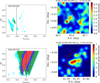Fig. 4.

Left panel: PPM plots for DES-RG 399 and 708. In each plot the vertical solid line shows the spectroscopic redshift of each radio source. Colored dots refer to significance levels >2σ (cyan), 3σ (green), 4σ (blue), 5σ (red), 6σ (brown), and 7σ (black). Right panel: Gaussian density maps centered at the projected space coordinates of the radio galaxies. The pixel size is 1/16 Mpc while the Gaussian kernel has σ = 3/16 Mpc. Sources with SDSS photometric redshifts between $z_{ov} - \bar{Δ z} / 2$ $z_{\mathrm{ov}}-\overline{\Delta z}/2$ and $z_{ov} + \bar{Δ z} / 2$ $z_{\mathrm{ov}}+\overline{\Delta z}/2$ were considered to produce the maps, where z_ov and $\bar{Δ z}$ $\overline{\Delta z}$ are reported in Table 7, for each overdensity. The solid black and dashed red circles are centered at the projected space coordinates of the radio source. The former has a (physical) radius of 1 Mpc, estimated at z_ov, while the latter, with a radius ℛ_PPM, denotes the region within which the PPM detects the overdensity. The dotted-dashed green circle is centered at the peak of the detection as found by the wavelet transform and has a radius ℛ_w.

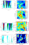Fig. 5.

PPM plots (left panel) and wavelet density maps (right panel) associated with COSMOS-FRI 16, 31, and 70. The color code is analogous to that of Fig. 4. We have used photometric redshifts from Laigle et al. (2016) for the fields of COSMOS-FRI 16 and 31, and from Ilbert et al. (2009) for the field of COSMOS-FRI 70.

4.3. The wavelet-based upgrade of the PPM

The PPM does not search for overdensities blindly, but relies on a positional prior, that is, the projected space coordinates of the radio galaxy. In particular the PPM exploits this positional prior to partially overcome the limitation due to low-number count statistics and shot noise, that usually affect distant cluster searches based on galaxy number counts. As stressed in Castignani et al. (2014a,b) such an exploitation is performed by privileging an accurate photometric redshift sampling to the detriment of a less sophisticated projected space tessellation.

In this work we aim at improving the ability of the method to locate and characterize the overdensity in the projected space, once its redshift is determined by the PPM. As further described in the following this improvement is made by applying a 2D wavelet transform.

For each overdensity, detected at a redshift z_ov, sources with photometric redshifts within $z_{ov} - \bar{Δ z} / 2$ $z_{\mathrm{ov}}-\overline{\Delta z}/2$ and $z_{ov} + \bar{Δ z} / 2$ $z_{\mathrm{ov}}+\overline{\Delta z}/2$ are considered. We used such sources to produce a 2D map with a pixel size of 1/16 Mpc. We then filtered the 2D map with the task mr_filter within the multiresolution package MR/1 (Starck et al. 1998). The mr_filter is based on the wavelet transform. We ran it to detect structures including a treatment of the Poisson noise and an iterative multiresolution thresholding down to 2σ, which is consistent with the value adopted by the PPM to define overdensities¹³. Such a wavelet-based procedure is similar to that used by the WaZP cluster finder (Benoist 2014; Dietrich et al. 2014).
From each wavelet map we then selected the highest peak falling within a circle centered at the projected coordinates of the radio galaxy and with a radius equal to ℛ_PPM. We define as θ_ov the projected separation (i.e., the miscentering) of the radio galaxy coordinates with respect to the overdensity peak, as found by mr_filter. This procedure aims at locating, in the projected space, the peak of the overdensity associated with the radio galaxy. For this reason, we limited the search to a circle of ℛ_PPM radius, which defines the overdensity found by the PPM. Extending the search to a larger region would possibly include peaks that are not physically associated with the radio galaxy. Distant (proto-)clusters can in fact exhibit a complex structure. For example, still-forming proto-clusters may extend up to ∼10 Mpc (see e.g., Overzier 2018, for a review).
A refinement of the estimate of the overdensity size is then derived as the minimum projected distance from the wavelet peak, selected as in the previous step, at which the wavelet map is reduced to one hundredth of the peak value. We denote such a size as ℛ_w.

5. Results

5.1. Stellar masses

For all five sources in our sample we estimated the stellar masses from the SEDs of Sect. 2.3 using a standard LePhare procedure, similarly to previous work (e.g., Laigle et al. 2016).

Stellar masses were estimated by fitting the photometric data points with synthetic templates of three elliptical galaxies from the PEGASE2 library (Fioc & Rocca-Volmerange 1997). A Rana & Basu (1992) initial mass function (IMF) was assumed.

Concerning COSMOS-FRI 16, 31, and 70, B13 report stellar masses of log(M/M_⋆) = 10.74, 10.75, and 10.65. They assumed several IMFs in their modeling (Salpeter 1955; Kroupa 2001; Chabrier 2003). From the results reported in Table 5 we observe that these mass estimates are fairly consistent with those estimated independently in this work. In fact stellar-mass estimates rely on stellar-population synthesis models and have statistical uncertainties of ∼(0.10−0.14) dex (e.g., Roediger & Courteau 2015). An additional uncertainty of ∼0.25 dex may be added because of the unknown IMF (Wright et al. 2017), yielding a typical uncertainty of ∼0.3 dex, which is adopted for all stellar masses estimated in this work and reported in Table 5.

Table 5.

Results of the SED modeling.

5.2. Star formation rates

By integrating the SED best-fit model for the dust between 8 and 1000 μm in the rest frame we derived an estimate for the FIR luminosity that we converted into an estimate for the star formation rate (SFR) using the Kennicutt (1998) relation. We denote such SFR estimates as SFR_SED, where the subscript SED stands for the fact that the SFR is estimated using the FIR SED best-fit model.

Our SFR_SED estimates are indeed upper limits, since in the FIR >24 μm observer frame domain we only have upper limits to the fluxes. Therefore we also estimated the SFRs using the available ∼24 μm (Spitzer MIPS or WISE W4) fluxes. We denote such SFR estimates as SFR_24 μm, where the subscript 24 μm refers to the fact that the SFR is estimated using the ∼24 μm fluxes. To estimate SFR_24 μm we adopted the same procedure described in Castignani et al. (2018) that is adapted from that of McDonald et al. (2016), as outlined below.

We estimated the λ = 24 μm rest-frame luminosities λL_λ from the observer-frame ∼24 μm fluxes by assuming a power-law model, L_λ ∝ λ^γ, with γ = 2.0 ± 0.5 (Casey 2012). We have incorporated the uncertainties in both γ and the observed 24 μm fluxes by using M = 100 000 values drawn from Gaussian distributions centered at the mean values and with standard deviations equal to the associated uncertainties. Subsequently, we adopted the Calzetti et al. (2007) relation to convert the 24 μm rest-frame luminosities into the SFR_24 μm estimates. The SFR_24 μm values and uncertainties were finally estimated as the medians and the 68.27% confidence levels derived from the M realizations, respectively.

For COSMOS-FRI 31, we only have upper limits in the FIR. We therefore derived a 3σ upper limit to the SFR_24 μm. Hereafter we adopt SFR_24 μm as our fiducial estimate for the SFR. The SFR_24 μm is in fact always lower than and therefore consistent with the SFR_SED upper limits.

Estimating the SFR from the observer frame 24 μm flux could be problematic for distant sources, because in the rest frame such a flux corresponds to the emission at shorter wavelengths, namely 24 μm/(1 + z), where z is the source redshift. Nevertheless, we stress that the observer frame 24 μm flux is adopted in the literature as a proxy for the SFR, in the absence of other SFR estimators, also for distant galaxies, such as in the recent work by Wang et al. (2018) on cluster galaxies at z ∼ 2.5 with detections in CO(1→0).

The specific SFR estimates for our sources are in overall agreement, within the reported uncertainties, with the empirical values by Speagle et al. (2014) for main sequence (MS) field galaxies with similar redshift and stellar mass, as reported in Table 5. We point out that our SFR estimates are also supported by a hint for a UV bump, possibly associated with star formation, observed by B13, in the SED of COSMOS-FRI 16, 31 and 70 (Fig. 3).

We stress that our radio sources, in particular DES-RG 399 and 708, have nearby companions clearly visible in their optical images (see e.g., Fig. 1), located at an angular separation consistent with the WISE and Spitzer MIPS positional accuracy of ∼6 arcsec. It is therefore possible that such companions might contaminate the observed IR emission, resulting in biased-high SFR estimates. Similarly, active galactic nucleus (AGN) torus and/or synchrotron emission could contaminate the observed FIR spectrum, even if at such wavelengths the AGN contribution is typically limited to ≲20% for distant star forming galaxies (Donley et al. 2012; Pozzi et al. 2012; Delvecchio et al. 2014). We also note that our photometric data set does not allow us to properly break the degeneracy between the synchrotron, torus, and dust emission.

5.3. Molecular gas properties

We describe in this section the results obtained with our IRAM-30 m observations. All our targets were unresolved by our observations, with a beam of ∼11 arcsec $(\frac{210 GHz}{ν_{obs}})$ $(\frac{210\,\mathrm{GHz}}{\nu_{\mathrm{obs}}})$ at observer frame frequency ν_obs (Kramer et al. 2013).

A hint of a tentative CO(7→6) detection is found at 2.2σ for COSMOS-FRI 70. In Fig. 6 we report the spectrum obtained for COSMOS-FRI 70 as well as an RGB image of the radio source and the IRAM-30 m field of view. Visual inspection of Fig. 6 (right) reveals several sources within the IRAM-30 m beam. Among them the galaxy with the smallest angular separation (i.e., 3.7 arcsec) from COSMOS-FRI 70 has a photometric redshift from the COSMOS2015 catalog (Laigle et al. 2016) equal to $z_{phot} = 2 . 07_{- 0.41}^{+ 0.09}$ $z_{\mathrm{phot}}=2.07^{+0.09}_{-0.41}$ , which is (marginally) consistent with the spectroscopic redshift of COSMOS-FRI 70, considering the large photometric redshift uncertainties. Here the subscript phot stands for photometric. We cannot exclude the possibility that the tentative CO(7→6) emission observed in the spectrum is due to our target COSMOS-FRI 70 and also possibly to its nearby companion, both unresolved by the IRAM-30 m. We stress that confirmation with higher-S/N data is needed, to claim a detection.

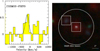Fig. 6.

Left panel: baseline-subtracted spectrum of COSMOS-FRI 70 obtained with the IRAM-30 m. The solid curve shows the Gaussian fit to the CO(7→6) emission line. In the y-axis we show T_mb in units of millikelvin. Right panel: RGB image centered at the coordinates of COSMOS-FRI 70 and obtained using Spitzer 3.6 μm (Sanders et al. 2007), Subaru r-, and Subaru B-band images (Taniguchi et al. 2007) for the R, G, and B channels, respectively. The two squares denote the locations of COSMOS-FRI 70 and its northern companion with $z_{phot} = 2 . 07_{- 0.41}^{+ 0.09}$ $z_{\mathrm{phot}}=2.07^{+0.09}_{-0.41}$ from the Laigle et al. (2016) catalog. The white circle shows the IRAM-30 m beam. North is up.

For the other four sources in the sample, DES-RG 399, DES-RG 708, COSMOS-FRI 16, and COSMOS-FRI 31, we reached rms noise levels for the antenna temperature (Ta^*) equal to 0.2, 0.2, 0.8, and 0.7 mK, respectively, within the entire 4 GHz bandwidth and at 300 km s⁻¹ resolution. We used the rms noise levels to set 3σ upper limits.

In Table 4 we report the results of our analysis, where standard efficiency corrections have been applied to convert i) Ta^* into the main beam temperature T_mb and then ii) T_mb into the corresponding CO line flux, where a 5 Jy K⁻¹ conversion is used.

In Table 4 we report 3σ upper limits to the total molecular gas mass for all five radio sources in our sample, including COSMOS-FRI 70, as described in the following.

5.3.1. Molecular gas mass

We derived the CO(J → J–1) luminosity L′_{CO(J → J − 1)} from the velocity integrated CO(J → J–1) flux S_{CO(J → J − 1)} Δv by using Eq. (3) of Solomon & Vanden Bout (2005):

$\begin{matrix} L_{CO (J \to J - 1)}^{'} = 3.25 \times 10^{7} S_{CO (J \to J - 1)} Δ v ν_{obs}^{- 2} D_{L}^{2} {(1 + z)}^{- 3}, \end{matrix}$ $\begin{aligned} L^\prime _{\rm CO(\textit{J}\rightarrow \textit{J}{-}1)}=3.25\times 10^7\,S_{\rm CO(\textit{J}\rightarrow \textit{J}{-}1)}\,\Delta v\, \nu _{\rm {obs}}^{-2}\,D_L^2\,(1+z)^{-3}, \end{aligned}$ (2)

where ν_obs is the observer frequency of the CO(J → J–1) transition, D_L is the luminosity distance, and z the redshift of the radio source.

By assuming a Galactic CO-to-H₂ conversion factor X_CO ≃ 2 × 10²⁰ cm⁻¹/(K km s⁻¹), that is, α_CO = 4.36 M_⊙ (K km s⁻¹ pc²)⁻¹, typical of MS galaxies (Solomon et al. 1997; Bolatto et al. 2013), we estimated the 3σ upper limits to the total molecular gas masses M(H₂) = α_COL′_{CO(1 → 0)} = α_COL′_{CO(J → J − 1)}/r_J1 for the five radio galaxies in our sample. Here r_J1 = L′_{CO(J → J − 1)}/L′_{CO(1 → 0)} is the excitation ratio. Concerning the CO(3→2), CO(4→3) and CO(7→6) lines considered in this work we have assumed the following fiducial excitation ratios, namely, r₃₁ = 0.55 (Devereux et al. 1994; Daddi et al. 2015), r₄₁ = 0.40 (Papadopoulos et al. 2000), r₇₁ = 0.39 (González-López et al. 2017), that are adopted in the literature for star forming galaxies.

5.3.2. Star formation, main sequence, and depletion time

Among the five radio sources in our sample COSMOS-FRI 70 is the only one for which a hint of detection in CO is reported, at 2.2σ. Interestingly, if we assume M(H₂) = (5.0 × 2.2)×10¹⁰ M_⊙ inferred by our observations and corresponding to the formal 3σ upper limit of M(H₂) < 6.6 × 10¹⁰ M_⊙ reported in Table 4, the $SFR (24 μ m) = (245_{- 112}^{+ 205}) M_{⊙}$ ${\mathrm{{SFR}}(24\,\mu\mathrm{m})}=(245^{+205}_{-112})\,M_\odot$ /yr estimated for COSMOS-FRI 70 (see Table 5) agrees, within the errorbars, with the SFR expected from standard M(H₂) versus SFR relations. We used the relation between M(H₂) and the IR luminosity for both MS and color-selected star forming galaxies at z ∼ 0.5−2.3 found by Daddi et al. (2010) as well as that of Kennicutt (1998) between the total FIR luminosity and the SFR. This procedure yields an SFR = (136 ± 104) M_⊙/yr, where the reported uncertainties take into account those estimated for M(H₂) that are summed in quadrature to fiducial ∼58%, that is, 0.25 dex, uncertainties associated with the calibration and the scatter of the adopted scaling relations (Daddi et al. 2010).

We used the SFRs and molecular-mass estimates to set 3σ upper limits to the depletion time scale, associated with the consumption of the molecular gas of the the radio sources in our sample, apart for COSMOS-FRI 31; this latter has upper limits to both M(H₂) and SFR_24 μm which did not allow us to estimate τ_dep or its upper limit. Similarly, we set 3σ upper limits to the M(H₂)/M_⋆ ratio for our radio sources.

For comparison we also estimated the depletion time τ_dep, MS and the molecular gas to stellar mass ratio $(\frac{M (H_{2})}{M_{⋆}})_{MS}$ $\big(\frac{M(\mathrm{H_2})}{M_\star}\big)_{\mathrm{MS}}$ for MS field galaxies with redshift and stellar mass equal to those of our target galaxies, as found using the empirical relations provided by Tacconi et al. (2018). Our results are summarized in Table 4, while in Table 6 we report additional properties of COSMOS-FRI 70 obtained with our IRAM-30 m observations.

Table 6.

Additional IRAM-30 m results for COSMOS-FRI 70.

5.3.3. Continuum emission

We also attempted to set an upper limit on the continuum emission of COSMOS-FRI 70 by using the available total 8 GHz bandwidth associated with the LI and LO channels of WILMA and FTS, respectively, for each polarization. COSMOS-FRI 70 is in fact the only source in our sample that is observed at a relatively short wavelength, in the rest frame, ∼372 μm, which is close to the S_ν dust emission peak at ∼100 μm in the rest frame. It is also the source for which we achieved the smallest rms noise with our IRAM-30 m observations. We obtained an rms of 0.1 mJy over the total 8 GHz bandwidth. The rms is about one order of magnitude lower than the absolute value of the observed baseline level, which is due to the atmospheric turbulence. Therefore we conclude that the faintness of our targets, combined with the significant intrinsic atmospheric instability at mm wavelengths, prevents us from setting robust upper limits to the continuum emission of our targets.

5.4. Molecular gas properties of distant (proto-)cluster galaxies

We compare the results found for our galaxies in terms of molecular gas content, SFR, and depletion time with those found by previous work on distant (proto-)cluster galaxies at redshifts of z ∼ 0.2−5. Similarly to previous work by Noble et al. (2017) and Castignani et al. (2018) we considered (proto-)cluster galaxies from the literature with estimates of both stellar and total gas masses, as well as estimates or upper limits to the SFR.

We considered stellar masses M_⋆ > 10¹⁰ M_⊙ and SFR < 6 SFR_MS, where SFR_MS is the SFR estimated using the empirical recipe by Speagle et al. (2014) for MS field galaxies of stellar mass and redshift equal to those of the galaxy considered. Including galaxies significantly above the MS might lead to biased-high molecular-gas-to-stellar-mass ratios. Such galaxies are also usually associated with lower values for α_CO; see for example Noble et al. (2017) and Castignani et al. (2018) for a discussion. As further outlined below most of the galaxies considered for the comparison, including our target galaxies, have SFR ≲ 3 SFR_MS, and are formally consistent with being on the MS. For the sake of completeness we did not discard the remaining sources with 3 < SFR/SFR_MS < 6, given also the large uncertainties associated with the SFR.

In the following we distinguish between galaxies at redshifts lower and higher than z ≃ 2, which usually denotes in the literature the fiducial separation between galaxy clusters and proto-clusters, respectively.

5.4.1. Cluster galaxies at 0.2 ≲ z ≲ 2.0

We considered CO detections of distant, that is, z ∼ 0.2−2, cluster galaxies at z ∼ 0.2 (Cybulski 2016); z ∼ 0.4−0.5 (Geach et al. 2011; Jablonka 2013); z ∼ 1.1−1.2 (Wagg et al. 2012,Castignani et al. 2018); z ∼ 1.5−1.7 (Aravena et al. 2012,Rudnick et al. 2017; Webb et al. 2017; Noble et al. 2017, 2019; Hayashi et al. 2018); and z ≃ 2.0 (Coogan et al. 2018). We also included the serendipitous CO detections reported by Kneissl et al. (2018) and associated with galaxies likely belonging to the cluster candidate PLCK C073.4–57.5 at z = 1.54.

Requiring SFR < 6 SFR_MS and M_⋆ > 10¹⁰ M_⊙ yields 52 sources over 16 clusters. In the following we consider proto-cluster galaxies at z > 2.

5.4.2. Cluster galaxies at 2 ≲ z ≲ 5

We searched the literature for CO detections of cluster galaxies at z > 2. To this aim we considered the list of detections reported in Dannerbauer et al. (2017). Namely, we include the proto-cluster galaxies with CO detections at z = 2.148 (Dannerbauer et al. 2017); z = 2.41 (Ivison et al. 2013); z = 2.51 (Tadaki et al. 2014); z = 4.05 (GN20 proto-cluster, Tan et al. 2014); z = 5.2 (galaxy HDF850.1, Walter et al. 2012); and z = 5.3 (AzTEC-3 proto-cluster, Riechers et al. 2010). For the cluster galaxy HDF850.1 at z = 5.2 we assumed the stellar-mass estimate M_⋆ = (1.3 ± 0.6) × 10¹¹ M_⊙ by Serjeant & Marchetti (2014).

Furthermore we also considered the Spider Web Galaxy, namely MRC 1138–262. It is a radio galaxy at z = 2.161 hosted in a proto-cluster, with CO(1→0) detection reported by Emonts et al. (2013, 2016) and M_⋆ ≃ 10¹² M_⊙ (Hatch et al. 2009), for which we assumed a fiducial uncertainty of ∼0.5 dex.

We considered also the following recent CO observations by Lee et al. (2017), Ginolfi et al. (2017), and Wang et al. (2018). Lee et al. (2017) detected in CO(3→2) a sample of seven galaxies associated with a proto-cluster at z = 2.49 around the powerful high-z radio galaxy 4C 23.56. Ginolfi et al. (2017) reported the CO(4→3) emission from Candels-5001, a massive galaxy (M_⋆ ∼ 1.9 × 10¹⁰ M_⊙) at z = 3.47 hosted in a proto-cluster candidate. Wang et al. (2018) found CO(1→0) in a sample of 14 galaxies belonging to CLJ1001, the most distant X-ray cluster, at z = 2.51. The authors do not report SFR estimates for these 14 sources. Therefore, consistently with the procedure adopted in this work, we converted the total IR luminosities reported by Wang et al. (2018) for the 14 sources into SFR estimates using the Kennicutt (1998) relation.

This procedure yielded 26 sources with SFR < 6 SFR_MS and M_⋆ > 10¹⁰ M_⊙, over seven (proto-)clusters at z > 2. We note that Ivison et al. (2013) reported CO(1→0) detections associated with four hyper-luminous IR galaxies belonging to the proto-cluster HATLAS J084933 at z = 2.41 and with an estimated SFR in the range ∼(640−3400) M_⊙/yr. We did not select such sources since they do not satisfy the SFR < 6 SFR_MS criterion. For the same reason we also excluded the sub-millimeter proto-cluster galaxy AzTEC at z = 5.3 and with an estimated SFR of ∼1800 M_⋆/yr (Riechers et al. 2010).

By combining together both z ≲ 2 and z ≳ 2 (proto-)cluster galaxies our selection yielded a total of 78 galaxies over 23 (proto-)clusters with CO detections from the literature. To them we have also added our 5 target radio galaxies in dense megaparsec-scale environment (see Sect. 5.5), implying a total of 83 galaxies over 28 (proto-)clusters.

We stress here that the cluster galaxy GAL0926+1242-B that i) belongs to the z = 0.49 cluster CL0926+1242, ii) has a stellar mass M_⋆ = 3.8 × 10⁹ M_⊙, and iii) has been detected in CO by Jablonka (2013) is the only source that was discarded because it does not satisfy the stellar mass criterion M_⋆ > 10¹⁰ M_⊙, despite having SFR < 6 SFR_MS.

5.4.3. Additional distant (proto-)cluster galaxies with CO detections

Additional z > 0.2 (proto-)cluster galaxies have been detected in CO by previous studies, but we have not included them in our analysis because they lack stellar-mass estimates from the literature. For the sake of completeness we list such sources in the following.

Casasola et al. (2013) detected CO(2→1) from an AGN belonging to a distant cluster around the powerful radio galaxy 7C 1756+6520 at z ≃ 1.4. The CO-emitting AGN is located at a projected separation of ∼0.8 Mpc from the radio galaxy. Interestingly, Ivison et al. (2012) detected CO(1→0) in two distant z ∼ 3−3.5 powerful radio galaxies (i.e., B3 J2330+3927 and 6C 1909+72) hosted in dense megaparsec-scale environment (Stevens et al. 2003). Hayatsu et al. (2017) detected a CO(9→8) emitter at z = 3.1, which was identified by the authors as a member of a known proto-cluster in the SSA22 region (Steidel et al. 1998). Oteo et al. (2018) and Miller et al. (2018) recently reported several CO detections in the core of two proto-clusters at z = 4.002 and z = 4.3, respectively.

5.4.4. Molecular gas diagrams

In Figs. 7 and 8 we report observational results concerning the aforementioned sample of 83 cluster galaxies from both the literature (78 sources) and this work (5 sources).

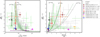Fig. 7.

Fractional offset from the star-forming MS as a function of the molecular gas depletion timescale (left panel) and molecular-gas-to-stellar-mass ratio (right panel); (proto-)cluster galaxies at 0.2 ≲ z ≲ 5 detected in CO are shown. In both panels the solid green curve shows the scaling relation for field galaxies found by Tacconi et al. (2018) for galaxies with log(M_⋆/M_⊙) = 11 and an effective radius equal to the mean value found by van der Wel et al. (2014) for star forming galaxies for given z and M_⋆. The green dashed lines show the statistical 1σ uncertainties in the model. The dotted black lines are the same scaling relation as the solid green lines, but for different stellar masses log(M/M_⋆) = 10.07 and 12, that represent the stellar mass range associated with the data points.

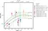Fig. 8.

Evolution of the molecular-gas-to-stellar-mass ratio as a function of the redshift for (proto-)cluster galaxies at 0.2 ≲ z ≲ 5 detected in CO. The color code is analogous to that of Fig. 7. The solid green curve is the scaling relation found by Tacconi et al. (2018) for field galaxies in the MS and with log(M_⋆/M_⊙) = 11, where an effective radius equal to the mean value found by van der Wel et al. (2014) for star forming galaxies for given z and M_⋆ is assumed. The green dashed lines show the statistical 1σ uncertainties in the model. The dotted black lines show the same scaling relation as the solid green line, but for different stellar masses log(M/M_⋆) = 10.07 and 12, that correspond to the stellar-mass range spanned by the data points.

In Fig. 7 we show the fractional offset from the star forming MS as a function of the molecular gas depletion timescale (left) and molecular-gas-to-stellar-mass ratio (right). In Fig. 8 we show the evolution of the molecular-gas-to-stellar-mass ratio.

In the left and right panels of Fig. 7 the x-axis values τ_dep and M(H₂)/M_⋆ have been rescaled by (1 + z)^B_t and η(z), respectively, to remove the redshift dependence, as estimated by Tacconi et al. (2018), where B_t = −0.62 and log η(z) = −3.62 × [log(1 + z)−0.66]².

We have corrected, where needed, the molecular mass estimates from the literature to take the different conversion factors α_CO into account. We have assumed α_CO = 4.36 M_⊙ (K km s⁻¹ pc²)⁻¹, in agreement with the value adopted in this work, while for each galaxy we have assumed the excitation level adopted in the corresponding work. Similarly to Castignani et al. (2018) we stress that by assuming the same α_CO we aim at having comparable molecular gas mass estimates for the galaxies considered. According to our SFR < 6 SFR_MS criterion the majority of the sources lie around the MS, which justifies the choice for α_CO.

In the figures we have color coded cluster galaxies at z ≲ 2 differently from those at z ≳ 2. We also highlight our five targets as well as, to the best of our knowledge, the most distant (proto-)BCGs detected in CO. They are i) the BCG at z = 1.7 observed in CO(2→1) by Webb et al. (2017), ii) the z = 1.99 BCG candidate of the cluster Cl J1449+0856 observed in both CO(4→3) and CO(3→2) by Coogan et al. (2018), iii) the proto-BCG candidate at z = 2.2, namely, MRC 1138–262, detected in CO(1→0) by Emonts et al. (2013, 2016) and, iv) the proto-BCG candidate Candels-5001 at z = 3.47 observed in CO(4→3) by Ginolfi et al. (2017).

In addition to Candels-5001 the other two CO detections reported in the figures at redshifts higher than that of COSMOS-FRI 70 and selected to have SFR < 6 SFR_MS are the galaxy GN20.2b at z = 4.0563 (Hodge et al. 2013; Tan et al. 2014) and HDF850.1 at z = 5.2 (Walter et al. 2012).

We stress here that the BCG candidate of the cluster Cl J1449+0856 at z = 2 was first described by Gobat et al. (2011) and has recently been observed with ALMA (Coogan et al. 2018; Strazzullo et al. 2018). No stellar mass estimate is reported for this source in these studies. However, an absolute K_s-band AB magnitude ∼20 is reported by Gobat et al. (2011) for the likely interacting triplet of galaxies associated with the proto-BCG. Following Gobat et al. (2011) we assumed a stellar-mass-to-light ratio of M_⋆/L_K_s = 3.8 M_⊙/L_⊙, where L_K_s is the rest frame K_s-band luminosity in units of the solar luminosity (L_⊙). This procedure yielded an estimate of the BCG stellar mass M_⋆ = (5.0 ± 2.7) × 10¹¹ M_⊙ which we have used in this work.

5.5. Megaparsec-scale overdensities

We searched for megaparsec-scale overdensities around the radio sources of our sample using the wPPM cluster-finder procedure and photometric redshifts of galaxies, as described in Sect. 4.

In Figs. 4 and 5 (right) we show the density maps corresponding to the overdensities associated with the radio sources. In the same figures we also show the peak and size (ℛ_w) of the detection as found by the wavelet transform. We also report in the same figures the PPM plots for the fields of the radio sources. For each pair (z_centroid; Δz) we have plotted the detection significance, where different colors correspond to different detection significances. Points with associated significance <2σ are not plotted. In each PPM plot the vertical solid line shows the spectroscopic redshift of the radio galaxy.

The wPPM results are summarized in Table 7. Megaparsec-scale overdensities with estimated core size in the range ∼(0.5–1) Mpc are found for all radio sources in our sample at redshifts consistent with the spectroscopic redshifts of the radio galaxies.

Table 7.

Properties of the megaparsec-scale overdensities around the radio sources.

5.5.1. DES-RG 399 and 708

We searched for overdensities around DES-RG 399 and 708 using photometric redshifts from the DR14 of SDSS, which has an AB magnitude limit of i ∼ 21.3. As a consistency check we verified that the cluster candidates around the two DES-RGs are both detected also when the deeper year 1 DES SN deep-field number 3 photometric redshift catalog (DES collaboration; C. Benoist, priv. comm.) is used. DES SN deep field photometry is in fact complete down to AB magnitudes i ∼ 24.5 and allowed us to detect both overdensities around DES-RG 399 and 708 at z_ov = 0.31 ± 0.05 and z_ov = 0.60 ± 0.05, with higher significance (3.8σ and 8.3σ) than that obtained using SDSS photometric redshifts, respectively.

We also searched for overdensities associated with DES-RG 399 and 708 within both RedMapper¹⁴ (v6.3, Rykoff et al. 2014) and Wen et al. (2012) cluster catalogs. Both catalogs were built using the SDSS photometric dataset and include cluster candidates up to z ≃ 0.8. Our search did not produce positive results, suggesting that the cluster candidates around DES-RG 399 and 708 might be associated with (rich) groups of more than massive ≳10¹⁴ M_⊙ clusters. In particular at the redshift of DES-RG 399 (z = 0.39) the completeness of the Wen et al. (2012) cluster catalog is estimated to be about ≃80%, while it drops significantly down to ≃30% at the redshift of DES-RG 708 (z = 0.61), for M₂₀₀ > 6 × 10¹³ cluster masses¹⁵.

5.5.2. COSMOS-FRI 16, 31, and 70

We searched for overdensities associated with COSMOS-FRI 16, 31, and 70 using the wPPM and photometric redshifts of galaxies from both Ilbert et al. (2009) and Laigle et al. (2016) photometric redshift catalogs. Overdensities associated with the COSMOS-FRIs are found for all three radio galaxies when the Ilbert et al. (2009) photometric redshift catalog is used. Cluster candidates associated with COSMOS-FRI 16 and 31 are also found when the Laigle et al. (2016) photometric redshift catalog is instead used. However the proto-cluster candidate around COSMOS-FRI 70 is found only when the Ilbert et al. (2009) photometric redshift catalog is adopted. This discrepancy might be due to different photometric selection associated with the Ilbert et al. (2009) and Laigle et al. (2016) catalogs. In Fig. 5 and Table 7 we report the results of our analysis for COSMOS-FRI 16 and 31, where the Laigle et al. (2016) catalog has been used, while for COSMOS-FRI 70 the results refer to the Ilbert et al. (2009) catalog.

5.6. Properties of the galaxies in the overdensities

In this section we aim to characterize the global properties of the galaxy population associated with the megaparsec-scale overdensities found around the radio galaxies in our sample. As outlined in the following a number of limitations prevent us from assigning (proto-)cluster membership using sophisticated probabilistic methods based on photometric redshifts of galaxies (e.g., Castignani & Benoist 2016; George et al. 2011). Cluster membership algorithms are usually applied to large samples of clusters/groups, that is, cluster membership derived with such methods has a statistical meaning. Limiting ourselves to the megaparsec-scale overdensities associated with the radio source in our sample, it is worth also noting that i) the (proto-)cluster structure and topology are complex and that ii) the estimated richness (N_selected) of the overdensities is relatively low. These two aspects limit us from applying accurate cluster membership assignments that take into account the cluster-centric distance of each galaxy (e.g., Rozo et al. 2009, 2015; Castignani & Benoist 2016). Furthermore defining the proto-cluster galaxies that will end up in a virialized cluster by z ∼ 0 is not a trivial task, as shown by Contini et al. (2016), based on semi-analytic simulations. More precisely they showed that the fraction of galaxies in the proto-cluster field that are not progenitors of z ∼ 0 cluster galaxies is not negligible, and about ∼(20−30)% for galaxies with M_⋆ ≃ 10⁹ M_⊙.

For these reasons we preferred to adopt a heuristic but still effective approach to select fiducial (proto-)cluster members, as described in the following. We verified a posteriori that this approach still gives reasonable and consistent results. Visual inspection of the density maps in Figs 4 and 5 (right) suggests that the overdensity peaks as found by the PPM and its wavelet-based upgrade are delimited within regions of similar size, that is, ℛ_PPM ≃ ℛ_w (see also Table 7). Furthermore, such regions are reasonably well contained within a circle centered at the radio galaxy coordinates and with a radius of 1 Mpc, which typically defines the cluster core size. We have therefore selected all galaxies within a projected distance of 1 Mpc from each radio source in our sample. The 1 Mpc radius was evaluated at the spectroscopic redshift z_RG of the radio source. Among such sources we then selected as fiducial (proto-)cluster members only those that have photometric redshifts within z_RG − σ₀ (1 + z_RG) and z_RG + σ₀ (1 + z_RG), with σ₀ = 0.03, which is consistent with the value adopted for the PPM procedure (see Sect. 4.2).

5.6.1. Color-magnitude and color-color plots

We made color-magnitude (CM) plots using the galaxies in the field of the radio galaxies, which were selected within a projected radius of 1 Mpc as described in the previous section. In particular we produced g-i versus i CM plots for sources in the field of DES-RG 399 and 708, using SDSS photometry. We also produced r-K_s versus K_s CM plots for sources in the field of COSMOS-FRI 16, 31, and 70 using available COSMOS r- and K_s-band photometry from the Suprime-CAM of Subaru (Taniguchi et al. 2007) and UltraVISTA (McCracken et al. 2012), respectively, derived from fixed 3″ aperture, as reported in Laigle et al. (2016). We note that the g- and i-band filters of SDSS have effective wavelengths equal to 4770 and 7625 Å. They were chosen because they optimally catch the 4000 Å break of DES-RG 399 and 708, which are redshifted at 5554 and 6423 Å, respectively. Similarly, the r- and K_s-band filters of Subaru Suprime-CAM and UltraVISTA have effective wavelengths equal to 6289 and 21 540 Å. The redshifted 4000 Å breaks of COSMOS-FRI 16, 31, and 70 optimally fall between these two wavelengths, being located at 7875, 7649, and 14 500 Å, respectively.

Concerning COSMOS-FRI 16, 31, and 70 we used their Subaru r- and CFHTLS K_s-band photometry from B13, consistently with what has been done for the SED modeling in Sect. 2.3. However we verified that using instead the photometric data from Laigle et al. (2016) does not change our final results.

The cluster candidates around DES-RG 399 and 708 have a small number of selected galaxies (see also Table 7). Therefore, we prefer not to show any CM plot for these overdensities. However by using the year 1 DES SN deep field number 3 photometric redshift catalog (DES collaboration; C. Benoist, priv. comm.) we verified that with the SDSS dataset we are indeed targeting only the bright end of the CM plot, that is, of the cluster galaxy luminosity function.

In Fig. 9 (left) we report the CM plots for sources in the field of COSMOS-FRI 16, 31, and 70, where two red-sequence models corresponding to formation redshifts z_f = 20 and 6.5 are overplotted and estimated using the Galaxy Evolutionary Synthesis Models (GalEv) tool¹⁶ (Kotulla et al. 2009). Model parameters are reported in Table 8 and are equal to those adopted by Kotyla et al. (2016), who studied the megaparsec-scale environments of distant radio sources.

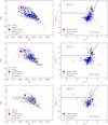Fig. 9.

Color-magnitude (left panel) and color-color (right panel) plots for sources within a projected distance of 1 Mpc from the COSMOS-FRI 16 (top panel), 31 (center panel), and 70 (bottom panel). Fiducial cluster members and COSMOS-FRI galaxies are distinguished from the remaining sources in the field. Left panel: red-sequence models for galaxies between 10¹⁰ and 5 × 10¹¹ M_⊙ are plotted. Red-sequence Models I and II correspond to a formation redshift z_f = 6.5 and 20, respectively. The horizontal dashed lines show a fiducial ±0.3 dex uncertainty in each model, similarly to Kotyla et al. (2016). Right panel: solid black line distinguishes between fiducial star-forming and quiescent galaxies, respectively. See text for further details.

Table 8.

GalEv parameters.

In the right panels of the same figure we also report the rest frame NUV-r versus r-J color-color plots for the same sources in the field of the COSMOS-FRI radio galaxies, as in the left panels. Such diagrams are commonly used in the literature to distinguish fiducial star-forming from quiescent galaxies (Williams et al. 2009; Laigle et al. 2016). Here NUV, r, and J denote magnitudes from GALEX, Subaru, and VISTA, respectively, from the Laigle et al. (2016) catalog.

5.6.2. Morphological classification

To investigate the morphology of our target COSMOS-FRI radio galaxies, we determined their half-light radius and Sèrsic index from high-resolution HST ACS F814W (I-band) images using Galfit (Peng et al. 2002, 2010). The pixel size of these images (see Fig. 2) is 0.03 arcsec, for an effective resolution of about 0.1 arcsec (∼0.8 kpc at the target redshifts). On the other hand we stress here that both SDSS and DES images have a resolution of ≲1 arcsec which does not allow us to optimally fit the light profile of DES-RG 399 and 708.

The Sèrsic law can be expressed as

$\begin{matrix} Σ (r) = Σ_{e} exp [b_{n} ({(\frac{r}{r_{e}})}^{1 / n} - 1)], \end{matrix}$ $\begin{aligned} \Sigma (r)=\Sigma _{\rm e}\exp \left[b_n\left(\left(\frac{r}{r_{\rm e}}\right)^{1/n}-1\right)\right], \end{aligned}$ (3)

where Σ(r) is the surface brightness at a projected distance r from the galaxy center, Σ_e is the surface brightness at the half-light radius r_e, n is the Sèrsic index, and b_n is a function of the Sèrsic index. The Sèrsic law with n = 4 fairly approximates the profile of classical elliptical galaxies, for which it holds b₄ = 7.669 (see e.g., Graham & Driver 2005, and references therein).

The fits were performed using a generic Tiny Tim (Krist 1995; Krist et al. 2011) point spread function for the HST ACS F814W filter, assuming a G2V stellar spectrum. Our Galfit analysis yielded n = 3.7 ± 0.2, 4.4 ± 0.1, and 4.3 ± 0.6, as well as r_e = (4.9 ± 0.8), (4.7 ± 0.8), and (2.9 ± 0.8) kpc for COSMOS-FRI 16, 31, and 70, respectively. The estimated Sèrsic indexes are consistent with those of elliptical galaxies (n = 4). The inferred effective radii r_e are fairly consistent with, albeit smaller than, those predicted by van der Wel et al. (2014) for MS galaxies of similar mass and redshift of COSMOS-FRI 16, 31, and 70, which are equal to 6.6, 6.6, and 4.8 kpc, respectively.

6. Discussion

The main goals of this work are to study the molecular gas associated with distant radio galaxies and to characterize their megaparsec-scale environments. To this aim we targeted CO with the IRAM-30 m telescope in five radio galaxies at z ∼ 0.4−2.6, which approximately corresponds to ∼7 Gyr of cosmic time. With more statistics, this will contribute to probing the cosmic history of molecular gas reservoirs in early-type (proto-)cluster core galaxies.

6.1. Molecular gas properties

6.1.1. Distant (proto-)BCG candidates with CO observations

We observed the five radio galaxies in our sample with the IRAM-30 m telescope, targeting several CO(J → J–1) lines, one per radio source and set upper limits to the total molecular gas mass for all five sources. However, a hint at 2.2σ of a possible detection of CO(7→6) is found for COSMOS-FRI 70, at z = 2.6. If confirmed with higher-S/N data it would become one of the most distant proto-BCG candidates detected in CO so far. In general, as further discussed in Sect. 6.2, the present study increases the statistics of CO observations in distant (proto-)BCG candidates.

In fact, as further mentioned in Sect. 5.4.4, to the best of our knowledge there are only a few distant (proto-)BCGs observed in CO with associated stellar-mass estimates. They are i) the cluster galaxy at z = 1.7 observed by Webb et al. (2017), ii) the BCG candidate at z = 1.99 of the cluster Cl J1449+0856 (Coogan et al. 2018), iii) MRC 1138–262 at z = 2.2 from Emonts et al. (2013, 2016), and iv) Candels-5001 at z = 3.472 (Ginolfi et al. 2017).

We point out here that our five distant radio galaxies were selected from among the ones with the strongest evidence of ongoing star formation within a total of ∼30 deg² comprising the COSMOS survey and the DES SN deep fields 2 and 3. Therefore, although distant star forming BCGs have been reported in previous studies (Webb et al. 2015a; McDonald et al. 2016; Bonaventura et al. 2017), our results suggest that large molecular gas reservoirs associated with them are rare.

6.1.2. Main sequence

The upper limits to the molecular gas content M(H₂)/M_⋆<0.11, 0.09, 1.8, 1.5, and 0.29 for the five sources in our sample at z = 0.4, 0.6, 0.91, 0.97, and 2.6, respectively, are consistent with the empirical values by Tacconi et al. (2018) for MS field galaxies. Similarly, the five radio galaxies have estimated depletion time upper limits in the range τ_dep ≲ (0.2−7) Gyr that are consistent with the values of MS galaxies, given the large uncertainties associated with both molecular gas mass and SFR estimates (see also Table 4 and Fig. 7).

We note that we assumed a Galactic α_CO conversion factor for all our target sources, typical of MS galaxies. Assuming a lower α_CO, typical of starburst galaxies (e.g., Bolatto et al. 2013, for a review), would lead to a lower molecular gas mass and a shorter depletion timescale.

The fact that our target sources are consistent with being on the MS suggest that they are not yet merging with their nearby galaxies. Concerning COSMOS-FRI 70, the spectrum reported in Fig. 6 implies an estimated FWHM = (225 ± 123) km for the CO(7→6) line. This FWHM supports the scenario where one single source is responsible for the observed tentative emission, despite the presence of nearby companions within the IRAM-30 m beam (Fig. 6, right).

However, the possibility of an interaction of the radio galaxies with their companions cannot be excluded, which is in agreement with previous studies that found that radio-loud AGNs are indeed in systems that are close to merging (Chiaberge et al. 2015). The interaction may lead to a starburst phase, as found for example in distant BCGs (z ≃ 1.7, Webb et al. 2017) as well as local major merging gas-rich pairs such as the Antennae Galaxies (Gao et al. 2001; Ueda et al. 2012; Whitmore et al. 2014). We also point out that we cannot exclude the presence of projection effects. We stress that deeper observations are needed to confirm the CO(7→6) emission and the line properties.

6.2. Megaparsec-scale overdensities around low-luminosity radio galaxies

In this section we discuss the properties of the megaparsec-scale environments associated with the radio galaxies in our sample. We show that our targets are indeed consistent with being among the most distant BCGs with constraints on their molecular gas mass.

Overdensities associated with all five radio galaxies in our sample were found by applying the wPPM, which uses the photometric redshift of galaxies.

6.2.1. Miscentering of the radio galaxies and morphology of the overdensities

Our wavelet-based analysis suggests that the overdensities have a complex morphology. DES-RG 708 at z = 0.61 is the only radio source which is found to be coincident in the projected space with its associated overdensity peak, namely a negligible 62 kpc miscentering is found. For the other four radio galaxies, a miscentering in the range ∼(0.3−1) Mpc is found, which suggests that the cluster candidates might not be fully relaxed or may still be forming. Interestingly, Ledlow & Owen (1995) found that ∼90% of the radio galaxies in local (z < 0.09) Abell clusters are within ∼200 kpc from the cluster center. Similarly, Smolčić et al. (2011) found that LLRGs with L_1.4 GHz ≃ 10^30.6−32 erg s⁻¹ Hz⁻¹ are preferentially located within 0.2 × r₂₀₀, that is, within ∼60 kpc from the center of X-ray selected groups up to z ∼ 1.3.

In Castignani et al. (2014a) we searched for overdensities around the parent sample of approximately 30 COSMOS-FRI radio galaxies from Chiaberge et al. (2009). We also used photometric redshifts from Ilbert et al. (2009). We found that some radio sources show evidence for a miscentering ≲120 kpc, while others show offsets of up to ∼500 kpc. The offsets were estimated comparing the projected coordinates of the COSMOS-FRIs with those of the fiducial centers of clusters and groups found in previous studies on the basis of X-ray emission and photometric/spectroscopic redshifts of galaxies (Finoguenov et al. 2007; George et al. 2011; Knobel et al. 2009, 2012; Diener et al. 2013).

In particular, the overdensities associated with COSMOS-FRI 16 and 31 are found in the Knobel et al. (2012) and Knobel et al. (2009) group catalogs, respectively, at an angular separation of 63 and 15 arcsec. Such offsets are not in full agreement with those found by the wPPM using photometric redshifts (see Table 7). We suggest that the discrepancy might be due to the different datasets used to select the cluster candidates. Knobel et al. (2009, 2012) used spectroscopic redshifts from the zCOSMOS-bright survey (Lilly et al. 2007) to search for overdensities. Such a discrepancy implies also that precise assessment of the center of the overdensity is in general difficult, especially in the case of low-richness systems, as in the case of our target galaxies (see Sect. 6.2.3).

We stress here that in the present work i) we have adapted the PPM to the specific case where the spectroscopic redshifts of the target radio galaxies are available (see Sect. 4.2) and ii) we have improved the PPM cluster finder by using a wavelet-based approach as described in Sect. 4.3. Therefore the results presented in this work supersede those of Castignani et al. (2014a), concerning COSMOS-FRI 16, 31, and 70. In the following we perform a comparison between such results.

6.2.2. Comments on the overdensity detections for COSMOS-FRI 16, 31, and 70

Limiting ourselves to the three COSMOS-FRI sources of this work, in Castignani et al. (2014a) we only found an overdensity, associated with COSMOS-FRI 16, at z_ov = 1.12 ± 0.06. The reason why no overdensity was found to be associated with the other two radio sources is that in Castignani et al. (2014a) we applied a smoothing procedure which allowed us to remove noisy features but also filtered-out low-S/N overdensities. This can be seen from visually inspecting the PPM plots of COSMOS-FRI 16, 31, and 70 shown in Appendix A of Castignani (2014). Low-S/N features, that is, those at ≳2σ, are visible in the PPM plots in Figs. 4 and 5, but they were conservatively not identified as cluster candidates by the PPM peak finding procedure in Castignani et al. (2014a) and Castignani (2014). The PPM was in fact originally conceived and applied to deal with photometric redshifts of the target radio galaxies, which increase the chance of having projection effects.

In this work we have optimized the PPM to the case where the spectroscopic redshifts of the radio galaxies are available. This was done mainly by i) applying no filtering procedure and ii) searching for an optimal redshift bin $\bar{Δ z}$ $\overline{\Delta z}$ at which the overdensity is detected in the PPM plot (see Sect. 4.2). Such improvements ultimately allowed us to effectively find overdensities around all three COSMOS-FRI sources in our sample. We also stress that COSMOS-FRI 16 is the only radio source in our sample for which two overdensities are detected in its field at a redshift consistent with that of the radio galaxy. For the sake of completeness both overdensities are shown in Fig. 5 and their estimated properties are reported in Table 7.

6.2.3. Low-richness structures

As mentioned above, in Castignani et al. (2014a) we also searched for overdensities associated with COSMOS-FRI sources using existing catalogs of clusters and groups. Limiting ourselves to COSMOS-FRI 16 and 31 at z < 1, the associated cluster candidates were found within the Knobel et al. (2012) and Knobel et al. (2009) group catalogs, respectively, with estimated masses of 1.9 × 10¹³ M_⊙ and 8.9 × 10¹² M_⊙.

The overdensity found with the wPPM around COSMOS-FRI 70 at z = 2.625 likely belongs to a (proto-)cluster. To the best of our knowledge this proto-cluster candidate has never been reported in previous work. If confirmed spectroscopically, it will be one of the most distant proto-clusters discovered around radio galaxies (see also e.g., Noirot et al. 2016, 2018). Castignani et al. (2014a) searched for overdensities associated with z > 1 COSMOS-FRI radio galaxies within the proto-cluster catalog of Diener et al. (2013), which was constructed using spectroscopic redshift information from the zCOSMOS-deep survey (Lilly et al. 2007, and in prep.). We found only one potential match, that is, COSMOS-FRI 03. In Castignani et al. (2014a) we also looked for cluster candidates using the Papovich (2008) method, which is based on overdensities of sources detected at 3.6 μm and 4.5 μm and is suited to search for (proto-)clusters at z > 1.3. Among the three COSMOS-FRI sources considered in this work, COSMOS-FRI 70 is the only one at z > 1.3. We did not find any overdensity associated with such a radio source using the Papovich (2008) method, which suggests that the overdensity around COSMOS-FRI 70 found by the wPPM might be consistent with those of rich groups.

Therefore, based on the results presented here, the megaparsec-scale overdensities around the LLRGs in our sample are likely associated with rich groups rather than massive ≳10¹⁴ M_⊙ clusters. Such a statement is also supported by the richness estimates provided by the wPPM. About N_selected ∼ (6−34) sources are in fact selected by the wPPM to detect the overdensities, with the only exception represented by the overdensity around COSMOS-FRI 16, for which ≳100 sources are selected.

We stress that spectroscopic follow-ups are ultimately needed to confirm the (proto-)cluster candidates around the radio sources in our sample and fully characterize their cluster population. Nevertheless, in the following section we discuss the properties of the galaxy population of our (proto-)cluster candidates using photometric redshift information.

6.2.4. Star forming (proto-)BCG candidates

We derived color-color and color-magnitude (CM) plots for galaxies within a projected distance of 1 Mpc from the radio galaxies (see Sect. 5.6 and Fig. 9). The colors and magnitudes of the three COSMOS-FRIs considered in this work are fairly consistent with model predictions for a red sequence of elliptical galaxies, independently of the formation redshift (z_f = 6.5, 20) associated with red-sequence models. COSMOS-FRI 70 has an r-K_s color that is formally redder than that predicted for the red sequence. However, the discrepancy might be still within the associated (large) model uncertainties, considering also the relatively high redshift z = 2.625 of COSMOS-FRI 70. In fact red-sequence modeling of distant (proto-)cluster galaxies might lead to results of which interpretation is difficult, even with the use of spectroscopic redshifts. We refer for example to Kotyla et al. (2016) and Noirot et al. (2016) who derived CM plots for galaxies around distant radio-loud AGNs in dense megaparsec-scale environments.

The three COSMOS-FRIs of this study are among the brightest galaxies in the corresponding (proto-)clusters. In particular COSMOS-FRI 70 is ∼0.3 mag brighter in the K_s band than the second-brightest fiducial proto-cluster member, within the 1 Mpc radius. These findings, associated with the high stellar masses, log(M/M_⊙) = 10.9−11.5, and the estimated Sèrsic indices, n ≃ 3.7−4.4, suggest that our target radio galaxies might be indeed associated with the (proto-)BCGs of the cluster candidates, or at least giant ellipticals in the cores of the clusters. Such a statement is also supported by the presence of nearby companions of our target radio galaxies, clearly visible in particular for DES-RG 399, DES-RG 708, and COSMOS-FRI 70 (Figs. 1, 6).

The rest frame NUV-r versus r-J color-color plots of the fiducial cluster members suggest that the great majority of the selected members around the COSMOS-FRIs show on-going star formation. This statement applies also to our target radio galaxies. COSMOS-FRI 16 and 31 are formally at the edge of the dividing line separating quiescent from star-forming galaxies, while COSMOS-FRI 70 is safely classified as a star-forming galaxy, according to the color-color plots. These results are consistent with those found by the SED modeling, which suggests that the three COSMOS-FRIs are indeed star forming, on the basis of their FIR and UV emission. The suggested star formation associated with the majority of the fiducial cluster galaxies, including the target radio galaxies, is not in contradiction with the possible presence of the red sequence, as suggested by the CM plots. In fact red but nevertheless star forming distant BCGs have been suggested also in recent studies (Bonaventura et al. 2017).

7. Summary and conclusions

We investigated the role of dense megaparsec-scale environment in processing molecular gas in LLRGs in the cores of galaxy (proto-)clusters. To this aim we selected a sample of five radio galaxies in the range z = 0.4−2.6 within the COSMOS survey and DES SN deep field number 3, as part of a search for distant radio galaxies with evidence of ongoing star formation on the basis of the FIR (WISE or Spitzer MIPS) emission at ∼24 μm. The radio sources have rest frame 1.4 GHz radio powers that are fairly consistent with those of LLRGs.

We targeted CO in the five LLRGs with IRAM-30 m and set upper limits on the total molecular gas mass for all five sources at z = 0.39, 0.61, 0.91, 0.97, and 2.6. We found M(H₂)/M_⋆ < 0.11, 0.09, 1.8, 1.5, and 0.29, respectively. For the most distant radio source, COSMOS-FRI 70 at z = 2.6, a hint of a tentative CO(7→6) emission is found at 2.2σ.

The upper limits to the molecular gas mass and the depletion time, τ_dep ≲ (0.2−7) Gyr, for the five LLRGs are in agreement with the values found for MS field galaxies (Tacconi et al. 2018) of similar mass and redshift.

We assembled and modeled the IR-to-UV SEDs for our targets and estimated their SFR and stellar mass in the range ≃(21−245) M_⊙/yr and log(M_⋆/M_⊙)≃(10.9−11.5), respectively, which are fairly consistent with empirical values by Speagle et al. (2014) for MS field galaxies.

We also searched for megaparsec-scale overdensities associated with the LLRGs using the Poisson Probability Method (PPM, Castignani et al. 2014b) and photometric redshifts of galaxies. The PPM has been upgraded in this work with an approach based on the wavelet-transform (wPPM). Overdensities are found for all five radio galaxies, at redshifts in agreement with the spectroscopic redshifts of the radio sources.

Our wavelet-based analysis suggests that the morphology of the megaparsec-scale overdensities is complex, typical of still-forming proto-clusters and not fully relaxed clusters. Our wPPM analysis, and the cross-matching of the LLRGs with existing cluster/group catalogs, also suggest that the detected overdensities are associated with rich (≲10¹⁴ M_⊙) groups.

Color-color and color-magnitude plots suggest that the LLRGs are star forming and on the high-luminosity tail of the red sequence. Our morphological analysis based on the HST ACS images (F814W filter) of the three COSMOS-FRIs in our sample at z = 0.91, 0.97, and 2.63 implies Sèrsic indices in the range n ≃ 3.7−4.4, which are typical of classical ellipticals and strengthen the proposed red-sequence scenario.

Our findings are in overall agreement with a scenario where the five LLRGs in our sample are (proto-)BCG candidates. The present study thus increases the still limited statistics of early-type galaxies in the cores of distant (proto-)clusters with CO observations. In particular, COSMOS-FRI 70 at z = 2.6, becomes one of the most distant BCG candidates with CO observations, while its associated proto-cluster candidate reported in this study is one of the most distant proto-clusters discovered around radio galaxies.

Higher-resolution and higher-surface-brightness-sensitivity observations will allow us to spatially resolve the radio galaxies in our sample from their nearby companions, to possibly distinguish between different gas-processing mechanisms (e.g., galaxy harassment, strangulation, ram-pressure, or tidal stripping), and to put tighter constraints on their molecular gas properties. The radio galaxies studied in this work are therefore excellent targets for ALMA as well as next-generation telescopes such as the James Webb Space Telescope.

¹

https://des.ncsa.illinois.edu/releases/dr1

²

http://www.sdss.org/dr14/

³

http://wise2.ipac.caltech.edu/docs/release/allwise/

⁴

https://irsa.ipac.caltech.edu/data/ISSA/index_cutouts.html

⁵

http://www.ukidss.org/surveys/surveys.html

⁶

http://www.sdss.org/dr14/spectro/sspp/#ExtinctionCalculations

⁷

http://www.sdss.org/dr14/algorithms/fluxcal/

⁸

http://galex.stsci.edu/GR6/

⁹

http://archive.eso.org/cms/eso-data/data-packages/zcosmos-data-release-dr1.html

¹⁰

Fanaroff & Riley (1974) originally reported an FR I/FR II radio-power divide of ∼2 × 10³² erg s⁻¹ Hz⁻¹ sr⁻¹ at 178 MHz, which we have converted to 1.4 GHz in the rest frame by assuming an isotropic emission and a radio spectral slope α = 0.8, as well as accounting for the different cosmology adopted by the authors.

¹¹

https://www.iram.fr/IRAMFR/GILDAS/

¹²

http://www.sdss.org/dr14/algorithms/photo-z/

¹³

The adopted mr_filter command is: “mr_filter -m 10 -i 3 -s 10.,3.,2.,2. -n 5 -f 3 -K -C 2 -p -e 0 -A input output”, where input and output denote the input and output.fits files corresponding to the original and wavelet-transformed maps, respectively.

¹⁴

http://risa.stanford.edu/redmapper/

¹⁵

Here M₂₀₀ is the mass enclosed by a radius encompassing the matter density 200 times the critical one.

¹⁶

http://www.galev.org

Acknowledgments

This work is based on observations carried out under project numbers 073-16 and 074-17 with the IRAM 30m telescope. IRAM is supported by INSU/CNRS (France), MPG (Germany) and IGN (Spain). We thank the anonymous referee for helpful comments that led to a substantial improvement of the paper. GC thanks Micol Bolzonella for helpful discussion about zCOSMOS-deep sources. GC and MC thank Colin Norman for the suggestion of using wavelet transforms in the PPM. PS acknowledges support from the ANR grant LYRICS (ANR-16-CE31-0011). This publication has made use of data products from the Infrared Astronomical Satellite (IRAS), Wide-field Infrared Survey Explorer (WISE), the UKIRT Infrared Deep Sky Survey (UKIDSS), the Sloan Digital Sky Survey (SDSS), the Dark Energy Survey (DES), the COSMOS survey, and the NASA/IPAC Extragalactic Database (NED). The WISE is a joint project of the University of California, Los Angeles, and the Jet Propulsion Laboratory/California Institute of Technology, funded by the National Aeronautics and Space Administration. Funding for the Sloan Digital Sky Survey IV has been provided by the Alfred P. Sloan Foundation, the U.S. Department of Energy Office of Science, and the Participating Institutions. SDSS-IV acknowledges support and resources from the Center for High-Performance Computing at the University of Utah. The SDSS web site is www.sdss.org. SDSS-IV is managed by the Astrophysical Research Consortium for the Participating Institutions of the SDSS Collaboration including the Brazilian Participation Group, the Carnegie Institution for Science, Carnegie Mellon University, the Chilean Participation Group, the French Participation Group, Harvard-Smithsonian Center for Astrophysics, Instituto de Astrofísica de Canarias, The Johns Hopkins University, Kavli Institute for the Physics and Mathematics of the Universe (IPMU)/University of Tokyo, Lawrence Berkeley National Laboratory, Leibniz Institut für Astrophysik Potsdam (AIP), Max-Planck-Institut für Astronomie (MPIA Heidelberg), Max-Planck-Institut für Astrophysik (MPA Garching), Max-Planck-Institut für Extraterrestrische Physik (MPE), National Astronomical Observatories of China, New Mexico State University, New York University, University of Notre Dame, Observatário Nacional/MCTI, The Ohio State University, Pennsylvania State University, Shanghai Astronomical Observatory, United Kingdom Participation Group,Universidad Nacional Autónoma de México, University of Arizona, University of Colorado Boulder, University of Oxford, University of Portsmouth, University of Utah, University of Virginia, University of Washington, University of Wisconsin, Vanderbilt University, and Yale University. Funding for the DES Projects has been provided by the U.S. Department of Energy, the US National Science Foundation, the Ministry of Science and Education of Spain, the Science and Technology FacilitiesCouncil of the United Kingdom, the Higher Education Funding Council for England, the National Center for Supercomputing Applications at the University of Illinois at Urbana-Champaign, the Kavli Institute of Cosmological Physics at the University of Chicago, the Center for Cosmology and Astro-Particle Physics at the Ohio State University, the Mitchell Institute for Fundamental Physics and Astronomy at Texas A&M University, Financiadora de Estudos e Projetos, Fundação Carlos Chagas Filho de Amparo à Pesquisa do Estado do Rio de Janeiro, Conselho Nacional de Desenvolvimento Científico e Tecnológico and the Ministério da Ciência, Tecnologia e Inovação, the Deutsche Forschungsgemeinschaft, and the Collaborating Institutions in the Dark Energy Survey. The Collaborating Institutions are Argonne National Laboratory, the University of California at Santa Cruz, the University of Cambridge, Centro de Investigaciones Energéticas, Medioambientales y Tecnológicas-Madrid, the University of Chicago, University College London, the DES-Brazil Consortium, the University of Edinburgh, the Eidgenössische Technische Hochschule (ETH) Zürich, Fermi National Accelerator Laboratory, the University of Illinois at Urbana-Champaign, the Institut de Ciències de l’Espai (IEEC/CSIC), the Institut de Física d’Altes Energies, Lawrence Berkeley National Laboratory, the Ludwig-Maximilians Universität München and the associated Excellence Cluster Universe, the University of Michigan, the National Optical Astronomy Observatory, the University of Nottingham, The Ohio State University, the OzDES Membership Consortium, the University of Pennsylvania, the University of Portsmouth, SLAC National Accelerator Laboratory, Stanford University, the University of Sussex, and Texas A&M University. Based in part on observations at Cerro Tololo Inter-American Observatory, National Optical Astronomy Observatory, which is operated by the Association of Universities for Research in Astronomy (AURA) under a cooperative agreement with the National Science Foundation. The NED is operated by the Jet Propulsion Laboratory, California Institute of Technology, under contract with the National Aeronautics and Space Administration.

References

Abbott, T. M. C., Abdalla, F. B., Allam, S., et al. 2018, ApJS, 239, 18 [NASA ADS] [CrossRef] [Google Scholar]
Alberts, S., Pope, A., Brodwin, M., et al. 2016, ApJ, 825, 72 [NASA ADS] [CrossRef] [Google Scholar]
Alloin, D., Barvainis, R., Guilloteau, S., et al. 2000, ApJ, 528, 81 [NASA ADS] [CrossRef] [Google Scholar]
Aravena, M., Carilli, C. L., Salvato, M., et al. 2012, MNRAS, 426, 258 [NASA ADS] [CrossRef] [Google Scholar]
Arnouts, S., Cristiani, S., Moscardini, L., et al. 1999, MNRAS, 310, 540 [NASA ADS] [CrossRef] [Google Scholar]
Baldi, R. D., Chiaberge, M., Capetti, A., et al. 2013, ApJ, 762, 30 [NASA ADS] [CrossRef] [Google Scholar]
Baldi, R. D., Giroletti, M., Capetti, A., et al. 2015, A&A, 574, A65 [NASA ADS] [CrossRef] [EDP Sciences] [Google Scholar]
Becker, R. H., White, R. L., & Helfand, D. J. 1995, ApJ, 450, 559 [NASA ADS] [CrossRef] [Google Scholar]
Benoist, C. 2014, Building the Euclid Cluster Survey – Scientific Program, Proceedings of a Conference held July 6–11 2014 at the Sexten Center for Astrophysics, 8 [Google Scholar]
Bolatto, A. T., Wolfire, M., Leroy, A. K., et al. 2013, ARA&A, 51, 207 [Google Scholar]
Bonaventura, N. R., Webb, T. M. A., Muzzin, A., et al. 2017, MNRAS, 469, 1259 [NASA ADS] [CrossRef] [Google Scholar]
Boulade, O., Charlot, X., Abbon, P., et al. 2003, SPIE, 4841, 72 [Google Scholar]
Brodwin, M., Stanford, S. A., Gonzalez, A. H., et al. 2013, ApJ, 779, 138 [NASA ADS] [CrossRef] [Google Scholar]
Calzetti, D., Kennicutt, R. C., Engelbracht, C. W., et al. 2007, ApJ, 666, 870 [NASA ADS] [CrossRef] [Google Scholar]
Capak, P., Aussel, H., Ajiki, M., et al. 2007, ApJS, 172, 99 [NASA ADS] [CrossRef] [Google Scholar]
Cardelli, J. A., Clayton, G. C., & Mathis, J. S. 1989, ApJ, 345, 245 [NASA ADS] [CrossRef] [Google Scholar]
Casali, M., Adamson, A., de Alves Oliveira, C., et al. 2007, A&A, 467, 777 [NASA ADS] [CrossRef] [EDP Sciences] [Google Scholar]
Casasola, V., Magrini, L., Combes, F., et al. 2013, A&A, 558, A60 [NASA ADS] [CrossRef] [EDP Sciences] [Google Scholar]
Casey, C. M. 2012, MNRAS, 425, 3094 [Google Scholar]
Castignani, G. 2014, Radio – Loud Active Galactic Nuclei from parsec to Mega-parsec scales, PhD Thesis, http://preprints.sissa.it/xmlui/handle/1963/7466 [Google Scholar]
Castignani, G., & Benoist, C. 2016, A&A, 595, A111 [NASA ADS] [CrossRef] [EDP Sciences] [Google Scholar]
Castignani, G., & De Zotti, G. 2015, A&A, 573, A125 [NASA ADS] [CrossRef] [EDP Sciences] [Google Scholar]
Castignani, G., Haardt, F., Lapi, A., et al. 2013, A&A, 560, A28 [NASA ADS] [CrossRef] [EDP Sciences] [Google Scholar]
Castignani, G., Chiaberge, M., Celotti, A., et al. 2014a, ApJ, 792, 114 [NASA ADS] [CrossRef] [Google Scholar]
Castignani, G., Chiaberge, M., Celotti, A., et al. 2014b, ApJ, 792, 113 [NASA ADS] [CrossRef] [Google Scholar]
Castignani, G., Combes, F., Salomé, P., et al. 2018, A&A, 617, A103 [NASA ADS] [CrossRef] [EDP Sciences] [Google Scholar]
Chabrier, G. 2003, PASP, 115, 763 [NASA ADS] [CrossRef] [Google Scholar]
Chary, R., & Elbaz, D. 2001, ApJ, 556, 562 [NASA ADS] [CrossRef] [Google Scholar]
Chiaberge, M., Tremblay, G., Capetti, A., et al. 2009, ApJ, 696, 1103 [NASA ADS] [CrossRef] [Google Scholar]
Chiaberge, M., Gilli, R., Lotz, J. M., et al. 2015, ApJ, 806, 147 [NASA ADS] [CrossRef] [Google Scholar]
Coleman, G. D., Wu, C. C., & Weedman, D. W. 1980, ApJS, 43, 393 [NASA ADS] [CrossRef] [Google Scholar]
Collins, C. A., Stott, J. P., Hilton, M., et al. 2009, Nature, 458, 603 [NASA ADS] [CrossRef] [PubMed] [Google Scholar]
Condon, J. J., Cotton, W. D., Greisen, E. W., et al. 1998, AJ, 115, 1693 [NASA ADS] [CrossRef] [Google Scholar]
Contini, E., De Lucia, G., Hatch, N., et al. 2016, MNRAS, 456, 1924 [NASA ADS] [CrossRef] [Google Scholar]
Coogan, R. T., Daddi, E., Sargent, M. T., et al. 2018, MNRAS, 479, 703 [NASA ADS] [Google Scholar]
Csabai, I., Dobos, L., Trencséni, M., et al. 2007, AN, 328, 852 [NASA ADS] [Google Scholar]
Cybulski, R. 2016, MNRAS, 459, 3287 [NASA ADS] [CrossRef] [Google Scholar]
Daddi, E., Elbaz, D., Walter, F., et al. 2010, ApJ, 714, L118 [Google Scholar]
Daddi, E., Dannerbauer, H., Liu, D., et al. 2015, A&A, 577, A46 [NASA ADS] [CrossRef] [EDP Sciences] [Google Scholar]
Dannerbauer, H., Lehnert, M. D., Emonts, B., et al. 2017, A&A, 608, A48 [NASA ADS] [CrossRef] [EDP Sciences] [Google Scholar]
Dawson, K. S., Schlegel, D. J., David, J., et al. 2013, AJ, 145, 10 [Google Scholar]
De Breuck, C., Neri, R., Morganti, R., et al. 2003a, A&A, 401, 911 [NASA ADS] [CrossRef] [EDP Sciences] [Google Scholar]
De Breuck, C., Neri, R., Omont, A., et al. 2003b, New Astron. Rev., 47, 285 [NASA ADS] [CrossRef] [Google Scholar]
De Breuck, C., Bertoldi, F., Carilli, C., et al. 2005, A&A, 430, 1 [NASA ADS] [CrossRef] [EDP Sciences] [Google Scholar]
Dekel, A., Birnboim, Y., Engel, G., et al. 2009a, Nature, 457, 451 [NASA ADS] [CrossRef] [PubMed] [Google Scholar]
Dekel, A., Sari, R., Ceverino, D., et al. 2009b, ApJ, 703, 785 [Google Scholar]
Delvecchio, I., Gruppioni, C., Pozzi, F., et al. 2014, MNRAS, 439, 2736 [NASA ADS] [CrossRef] [Google Scholar]
Devereux, N., Taniguchi, Y., Sanders, D. B., et al. 1994, AJ, 107, 2006 [NASA ADS] [CrossRef] [Google Scholar]
The Dark Energy Survey Collaboration 2005, ArXiv e-prints [arXiv:0510346] [Google Scholar]
The Dark Energy Survey Collaboration 2016, MNRAS, 460, 1270 [NASA ADS] [CrossRef] [Google Scholar]
Diener, C., Lilly, S. J., Knobel, C., Zamorani, G., et al. 2013, ApJ, 765, 109 [NASA ADS] [CrossRef] [Google Scholar]
Dietrich, J. P., Zhang, Y., Song, J., et al. 2014, MNRAS, 443, 1713 [NASA ADS] [CrossRef] [Google Scholar]
Donley, J. L., Koekemoer, A. M., Brusa, M., et al. 2012, ApJ, 748, 142 [NASA ADS] [CrossRef] [Google Scholar]
Donoso, E., Best, P. N., & Kauffmann, G. 2009, MNRAS, 392, 617 [NASA ADS] [CrossRef] [Google Scholar]
Edge, A. C. 2001, MNRAS, 328, 762 [NASA ADS] [CrossRef] [Google Scholar]
Emonts, B. H. C., Feain, I., Mao, M. Y., et al. 2011, ApJ, 734, 25 [NASA ADS] [CrossRef] [Google Scholar]
Emonts, B. H. C., Feain, I., Röttgering, H. J. A., et al. 2013, MNRAS, 430, 3465 [NASA ADS] [CrossRef] [Google Scholar]
Emonts, B. H. C., Lehnert, M. D., Villar-Martín, M., et al. 2016, Science, 354, 1128 [NASA ADS] [CrossRef] [Google Scholar]
Evans, A. S., Mazzarella, J. M., Surace, J. A., et al. 2005, ApJS, 159, 197 [NASA ADS] [CrossRef] [Google Scholar]
Fanaroff, B. L., & Riley, J. M. 1974, MNRAS, 167, 31 [NASA ADS] [CrossRef] [Google Scholar]
Finoguenov, A., Guzzo, L., Hasinger, G., et al. 2007, ApJS, 172, 182 [NASA ADS] [CrossRef] [Google Scholar]
Fioc, M., & Rocca-Volmerange, B. 1997, A&A, 326, 950 [NASA ADS] [Google Scholar]
Fraser-McKelvie, A., Brown, M. J. I., & Pimbblet, K. A. 2014, MNRAS, 444, 63 [Google Scholar]
Gao, Y., Lo, K. Y., Lee, S.-W., et al. 2001, ApJ, 548, 172 [NASA ADS] [CrossRef] [Google Scholar]
Geach, J. E., Smail, I., Moran, S. M., et al. 2011, ApJ, 730, L19 [NASA ADS] [CrossRef] [Google Scholar]
George, M. R., Leauthaud, A., Bundy, K., et al. 2011, ApJ, 742, 125 [NASA ADS] [CrossRef] [Google Scholar]
Ginolfi, M., Maiolino, R., Nagao, T., et al. 2017, MNRAS, 468, 3468 [NASA ADS] [CrossRef] [Google Scholar]
Gobat, R., Daddi, E., Onodera, M., et al. 2011, A&A, 526, A133 [NASA ADS] [CrossRef] [EDP Sciences] [Google Scholar]
González-López, J., Bauer, F. E., Aravena, M., et al. 2017, A&A, 608, A138 [NASA ADS] [CrossRef] [EDP Sciences] [Google Scholar]
Graham, A. W., & Driver, S. P. 2005, PASA, 22, 118 [NASA ADS] [CrossRef] [Google Scholar]
Greve, T. R., Ivison, R. J., & Papadopoulos, P. P. 2004, A&A, 419, 99 [NASA ADS] [CrossRef] [EDP Sciences] [Google Scholar]
Hambly, N. C., Collins, R. S., Cross, N. J. G., et al. 2008, MNRAS, 384, 637 [NASA ADS] [CrossRef] [Google Scholar]
Hamer, S. L., Edge, A. C., Swinbank, A. M., et al. 2012, MNRAS, 421, 3409 [NASA ADS] [CrossRef] [Google Scholar]
Hatch, N. A., Overzier, R. A., Kurk, J. D., et al. 2009, MNRAS, 395, 114 [NASA ADS] [CrossRef] [Google Scholar]
Hausman, M. A., & Ostriker, J. P. 1978, ApJ, 224, 320 [NASA ADS] [CrossRef] [Google Scholar]
Hayashi, M., Tadaki, K., Kodama, T., et al. 2018, ApJ, 856, 118 [NASA ADS] [CrossRef] [Google Scholar]
Hayatsu, N. H., Matsuda, Y., Umehata, H., et al. 2017, PASJ, 69, 45 [NASA ADS] [CrossRef] [Google Scholar]
Helou, G., & Walker, D. W. 1988, IRAS, 7, 1 [Google Scholar]
Hewett, P. C., Warren, S. J., Leggett, S. K., et al. 2006, MNRAS, 367, 454 [NASA ADS] [CrossRef] [Google Scholar]
Hill, G. J., & Lilly, S. J. 1991, ApJ, 367, 1 [NASA ADS] [CrossRef] [Google Scholar]
Hodge, J. A., Karim, A., Smail, I., et al. 2013, ApJ, 768, 91 [NASA ADS] [CrossRef] [Google Scholar]
Hodgkin, S. T., Irwin, M. J., Hewett, P. C., et al. 2009, MNRAS, 394, 675 [NASA ADS] [CrossRef] [Google Scholar]
Ilbert, O., Arnouts, S., McCracken, H. J., et al. 2006, A&A, 457, 841 [NASA ADS] [CrossRef] [EDP Sciences] [Google Scholar]
Ilbert, O., Capak, P., Salvato, M., et al. 2009, ApJ, 690, 1236 [NASA ADS] [CrossRef] [Google Scholar]
Ineson, J., Croston, J. H., Hardcastle, M. J., et al. 2013, ApJ, 770, 136 [NASA ADS] [CrossRef] [Google Scholar]
Ivison, R. J., Morrison, G. E., Biggs, A. D., et al. 2008, MNRAS, 390, 1117 [NASA ADS] [CrossRef] [Google Scholar]
Ivison, R. J., Smail, I., Papadopoulos, P. P., et al. 2011, MNRAS, 412, 1913 [NASA ADS] [CrossRef] [Google Scholar]
Ivison, R. J., Smail, I., Amblard, A., et al. 2012, MNRAS, 425, 1320 [NASA ADS] [CrossRef] [Google Scholar]
Ivison, R. J., Swinbank, A. M., Smail, I., et al. 2013, ApJ, 772, 137 [NASA ADS] [CrossRef] [Google Scholar]
Jablonka, P. 2013, A&A, 557, A103 [NASA ADS] [CrossRef] [EDP Sciences] [Google Scholar]
Jarrett, T. H., Cohen, M., Masci, F., et al. 2011, ApJ, 735, 112 [NASA ADS] [CrossRef] [Google Scholar]
Kennicutt, R. C. J. 1998, ARA&A, 36, 189 [Google Scholar]
Kessler, R., Marriner, J., Childress, M., et al. 2015, AJ, 150, 172 [NASA ADS] [CrossRef] [Google Scholar]
Klamer, I. J., Ekers, R. D., Sadler, E. M., et al. 2005, ApJ, 621, 1 [NASA ADS] [CrossRef] [Google Scholar]
Kneissl, R., Maria del Carmen, P., Martinache, C., et al. 2018, A&A, submitted [arXiv:1804.06581] [Google Scholar]
Knobel, C., Lilly, S. J., Iovino, A., et al. 2009, ApJ, 697, 1842 [NASA ADS] [CrossRef] [Google Scholar]
Knobel, C., Lilly, S. J., Iovino, A., et al. 2012, ApJ, 753, 121 [NASA ADS] [CrossRef] [Google Scholar]
Koekemoer, A. M., Aussel, H., Calzetti, D., et al. 2007, ApJS, 172, 196 [NASA ADS] [CrossRef] [Google Scholar]
Kotulla, R., Fritze, U., Weilbacher, P., et al. 2009, MNRAS, 396, 462 [NASA ADS] [CrossRef] [Google Scholar]
Kotyla, J. P., Chiaberge, M., Baum, S., et al. 2016, ApJ, 826, 46 [NASA ADS] [CrossRef] [Google Scholar]
Kramer, C., Penalver, J., Greve, A., et al. 2013, Improvement of the IRAM 30m Telescope Beam Pattern, www.iram-institute.org/medias/uploads/eb2013-v8.2.pdf [Google Scholar]
Krist, J. 1995, ASPC, 77, 349 [Google Scholar]
Krist, J. E., Hook, R. N., & Stoehr, F. 2011, Proc. SPIE, 8127, 81270J [CrossRef] [Google Scholar]
Kroupa, P. 2001, MNRAS, 322, 231 [NASA ADS] [CrossRef] [Google Scholar]
Laigle, C., McCracken, H. J., Ilbert, O., et al. 2016, ApJS, 224, 24 [NASA ADS] [CrossRef] [Google Scholar]
Larson, R. B., Tinsley, B. M., Caldwell, N., et al. 1980, ApJ, 237, 69 [Google Scholar]
Lauer, T. R., Gebhardt, K., Faber, S. M., et al. 2014, ApJ, 797, 82 [Google Scholar]
Lawrence, A., Warren, S. J., Almaini, O., et al. 2007, MNRAS, 379, 1599 [NASA ADS] [CrossRef] [MathSciNet] [Google Scholar]
Ledlow, M. J., & Owen, F. N. 1995, AJ, 109, 853 [NASA ADS] [CrossRef] [Google Scholar]
Lee, N., Le Floc’h, E., Sanders, D. P., et al. 2010, ApJ, 717, 175 [NASA ADS] [CrossRef] [Google Scholar]
Lee, M. M., Tanaka, I., Kawabe, R., et al. 2017, ApJ, 842, 55 [CrossRef] [Google Scholar]
Lidman, C., Suherli, J., Muzzin, A., et al. 2012, MNRAS, 427, 550 [NASA ADS] [CrossRef] [Google Scholar]
Lilly, S. J., Le Fevre, O., Renzini, A., et al. 2007, ApJS, 172, 70 [NASA ADS] [CrossRef] [Google Scholar]
Lim, J., Leon, S., Combes, F., et al. 2000, ApJ, 545, L93 [NASA ADS] [CrossRef] [Google Scholar]
Lim, J., Leon, S., Combes, F., & Trung, D.-V. 2004, ASSL, 319, 783 [NASA ADS] [Google Scholar]
Mauch, T., & Sadler, E. M. 2007, MNRAS, 375, 931 [NASA ADS] [CrossRef] [Google Scholar]
McCracken, H. J., Milvang-Jensen, B., Dunlop, J., et al. 2012, A&A, 544, A156 [NASA ADS] [CrossRef] [EDP Sciences] [Google Scholar]
McDonald, M., Stalder, B., Bayliss, M., et al. 2016, ApJ, 817, 86 [NASA ADS] [CrossRef] [Google Scholar]
McNamara, B. R., Russell, H. R., et al. 2014, ApJ, 785, 44 [NASA ADS] [CrossRef] [Google Scholar]
Miley, G., & De Breuck, C. 2008, A&ARv, 15, 67 [NASA ADS] [CrossRef] [Google Scholar]
Miller, T. B., Chapman, S. C., Aravena, M., et al. 2018, Nature, 556, 469 [NASA ADS] [CrossRef] [Google Scholar]
Moore, B., Lake, G., Quinn, T., et al. 1999, MNRAS, 304, 465 [NASA ADS] [CrossRef] [Google Scholar]
Morrissey, P., Conrow, T., Barlow, T. A., et al. 2007, ApJS, 173, 682 [NASA ADS] [CrossRef] [Google Scholar]
Moshir, M., Kopan, G., Conrow, T., et al. 1990, BAAS, 22, 1325 [Google Scholar]
Nesvadba, N. P. H., Neri, R., De Breuck, C., et al. 2009, MNRAS, 395, 16 [Google Scholar]
Noble, A. G., McDonald, M., Muzzin, A., et al. 2017, ApJ, 842, 21 [CrossRef] [Google Scholar]
Noble, A. G., Muzzin, A., McDonald, M., et al. 2019, ApJ, 870, 56 [NASA ADS] [CrossRef] [Google Scholar]
Noirot, G., Vernet, J., De Breuck, C., et al. 2016, ApJ, 830, 90 [NASA ADS] [CrossRef] [Google Scholar]
Noirot, G., Stern, D., Mei, S., et al. 2018, ApJ, 859, 38 [NASA ADS] [CrossRef] [Google Scholar]
Ocaña Flaquer, B., Combes, F., Lim, J., et al. 2010, A&A, 518, A90 [NASA ADS] [CrossRef] [EDP Sciences] [Google Scholar]
Ocvirk, P., Pichon, C., Teyssier, R., et al. 2008, MNRAS, 390, 1326 [NASA ADS] [Google Scholar]
O’Donnell, J. E. 1994, ApJ, 422, 158 [NASA ADS] [CrossRef] [Google Scholar]
Oteo, I., Ivison, R. J., Negrello, M., et al. 2018, ApJ, 856, 720 [NASA ADS] [Google Scholar]
Overzier, R. A. 2018, A&ARv, 24, 140 [Google Scholar]
Papadopoulos, P. P., Röttgering, H. J. A., van der Werf, P. P., et al. 2000, ApJ, 528, 626 [NASA ADS] [CrossRef] [Google Scholar]
Papovich, C. 2008, ApJ, 676, 206 [NASA ADS] [CrossRef] [Google Scholar]
Paterno-Mahler, R., Blanton, E. L., Brodwin, M., et al. 2017, ApJ, 844, 78 [NASA ADS] [CrossRef] [Google Scholar]
Peng, C. Y., Ho, L. C., Impey, C. D., et al. 2002, AJ, 124, 266 [NASA ADS] [CrossRef] [Google Scholar]
Peng, C. Y., Ho, L. C., Impey, C. D., et al. 2010, AJ, 139, 2097 [NASA ADS] [CrossRef] [Google Scholar]
Planck Collaboration VI. 2018, A&A, submitted [arXiv:1807.06209] [Google Scholar]
Pozzi, F., Vignali, C., Gruppioni, C., et al. 2012, MNRAS, 423, 1909 [NASA ADS] [CrossRef] [Google Scholar]
Prescott, M. K. M., Impey, C. D., Cool, R. J., et al. 2006, ApJ, 644, 100 [NASA ADS] [CrossRef] [Google Scholar]
Rana, N. C., & Basu, S. 1992, A&A, 265, 499 [NASA ADS] [Google Scholar]
Riechers, D. A., Capak, P. L., Carilli, C. L., et al. 2010, ApJ, 720, 131 [Google Scholar]
Riess, A. G., Macri, L. M., Hoffmann, S. L., et al. 2016, ApJ, 826, 56 [NASA ADS] [CrossRef] [Google Scholar]
Riess, A. G., Casertano, S., Yuan, W., et al. 2018, ApJ, 855, 136 [NASA ADS] [CrossRef] [Google Scholar]
Roediger, J. C., & Courteau, S. 2015, MNRAS, 452, 3209 [NASA ADS] [CrossRef] [Google Scholar]
Rozo, E., Rykoff, E. S., Koester, B. P., et al. 2009, ApJ, 703, 601 [NASA ADS] [CrossRef] [Google Scholar]
Rozo, E., Rykoff, E. S., Becker, M., et al. 2015, MNRAS, 453, 38 [NASA ADS] [CrossRef] [Google Scholar]
Rudnick, G., Hodge, J., Walter, F., et al. 2017, ApJ, 849, 27 [NASA ADS] [CrossRef] [Google Scholar]
Russell, H. R., McNamara, B. R., Edge, A. C., et al. 2014, ApJ, 784, 78 [NASA ADS] [CrossRef] [Google Scholar]
Rykoff, E. S., Rozo, E., Busha, M. T., et al. 2014, ApJ, 785, 104 [NASA ADS] [CrossRef] [Google Scholar]
Salomé, P., & Combes, F. 2003, A&A, 412, 657 [NASA ADS] [CrossRef] [EDP Sciences] [Google Scholar]
Salomé, P., Combes, F., Edge, A. C., et al. 2006, A&A, 454, 437 [NASA ADS] [CrossRef] [EDP Sciences] [Google Scholar]
Salpeter, E. E. 1955, ApJ, 121, 161 [Google Scholar]
Sanders, D. B., Salvato, M., Aussel, H., et al. 2007, ApJS, 172, 86 [Google Scholar]
Schinnerer, E., Smolić, V., Carilli, C. L., et al. 2007, ApJS, 172, 46 [NASA ADS] [CrossRef] [Google Scholar]
Schlafly, E. F., & Finkbeiner, D. P. 2011, ApJ, 737, 103 [NASA ADS] [CrossRef] [Google Scholar]
Scoville, N. Z., Yun, M. S., Windhorst, R. A., et al. 1997, ApJ, 485, 21 [NASA ADS] [CrossRef] [Google Scholar]
Scoville, N., Aussel, H., Benson, A., et al. 2007, ApJS, 172, 1 [NASA ADS] [CrossRef] [Google Scholar]
Serjeant, S., & Marchetti, L. 2014, MNRAS, 443, 3118 [NASA ADS] [CrossRef] [Google Scholar]
Smolčić, V., Zamorani, G., Schinnerer, E., et al. 2009, ApJ, 696, 24 [NASA ADS] [CrossRef] [Google Scholar]
Smolčić, V., Finoguenov, A., Zamorani, G., et al. 2011, MNRAS, 416, L31 [NASA ADS] [CrossRef] [Google Scholar]
Snellen, I. A. G., & Best, P. N. 2001, MNRAS, 328, 897 [NASA ADS] [CrossRef] [Google Scholar]
Solomon, P. M., & Vanden Bout, P. A. 2005, ARA&A, 43, 677 [NASA ADS] [CrossRef] [Google Scholar]
Solomon, P. M., Downes, D., Radford, S., et al. 1997, ApJ, 478, 144 [NASA ADS] [CrossRef] [Google Scholar]
Speagle, J. S., Steinhardt, C. L., Capak, P. L., et al. 2014, ApJS, 214, 15 [NASA ADS] [CrossRef] [Google Scholar]
Starck, J.-L., Murtagh, F. D., & Bijaoui, A. 1998, Image Processing and Data Analysis (New York: Cambridge University Press), 297 [Google Scholar]
Steidel, C. C., Adelberger, K. L., Dickinson, M., et al. 1998, ApJ, 492, 428 [NASA ADS] [CrossRef] [Google Scholar]
Stevens, J. A., Ivison, R. J., Dunlop, J. S., et al. 2003, Nature, 425, 264 [NASA ADS] [CrossRef] [PubMed] [Google Scholar]
Stott, J. P., Collins, C. A., Burke, C., et al. 2011, MNRAS, 414, 445 [NASA ADS] [CrossRef] [Google Scholar]
Stott, J. P., Hickox, R. C., Edge, A. C., et al. 2012, MNRAS, 422, 2213 [NASA ADS] [CrossRef] [Google Scholar]
Strazzullo, V., Coogan, R. T., Daddi, E., et al. 2018, ApJ, 862, 64 [NASA ADS] [CrossRef] [Google Scholar]
Tacconi, L. J., Genzel, R., Saintonge, A., et al. 2018, ApJ, 853, 179 [NASA ADS] [CrossRef] [Google Scholar]
Tadaki, K., Kodama, T., Tanaka, I., et al. 2014, ApJ, 788, 23 [NASA ADS] [CrossRef] [Google Scholar]
Tan, Q., Daddi, E., Magdis, G., et al. 2014, A&A, 569, A98 [NASA ADS] [CrossRef] [EDP Sciences] [Google Scholar]
Taniguchi, Y., Scoville, N., Murayama, T., et al. 2007, ApJS, 172, 9 [NASA ADS] [CrossRef] [Google Scholar]
Tremblay, G. R., Oonk, J. B. R., Combes, F., et al. 2016, Nature, 534, 218 [NASA ADS] [CrossRef] [Google Scholar]
Trump, J. R., Impey, C. D., McCarthy, P. J., et al. 2007, ApJS, 172, 383 [NASA ADS] [CrossRef] [Google Scholar]
Ueda, J., Iono, D., Petitpas, G., et al. 2012, ApJ, 745, 65 [NASA ADS] [CrossRef] [Google Scholar]
van der Wel, A., Franx, M., van Dokkum, P. G., et al. 2014, ApJ, 788, 28 [NASA ADS] [CrossRef] [Google Scholar]
von der Linden, A., Best, P. N., Kauffmann, G., et al. 2007, MNRAS, 379, 867 [NASA ADS] [CrossRef] [Google Scholar]
Wagg, J., Pope, A., Alberts, S., et al. 2012, ApJ, 752, 91 [NASA ADS] [CrossRef] [Google Scholar]
Walter, F., Decarli, R., Carilli, C., et al. 2012, Nature, 486, 233 [NASA ADS] [CrossRef] [Google Scholar]
Wang, T., Elbaz, D., Daddi, E., et al. 2018, ApJ, 867, 29 [CrossRef] [Google Scholar]
Webb, T. M. A., O’Donnell, D., Yee, H. K. C., et al. 2013, AJ, 146, 84 [NASA ADS] [CrossRef] [Google Scholar]
Webb, T. M. A., Muzzin, A., Noble, A., et al. 2015a, ApJ, 814, 96 [NASA ADS] [CrossRef] [Google Scholar]
Webb, T. M. A., Muzzin, A., Noble, A., et al. 2015b, ApJ, 809, 173 [NASA ADS] [CrossRef] [Google Scholar]
Webb, T. M. A., Lowenthal, J., Yun, M., et al. 2017, ApJ, 844, 17 [NASA ADS] [CrossRef] [Google Scholar]
Wen, Z. L., Han, J. L., Liu, F. S., et al. 2012, ApJS, 199, 34 [NASA ADS] [CrossRef] [Google Scholar]
White, S. D. M. 1976, MNRAS, 177, 717 [NASA ADS] [CrossRef] [Google Scholar]
Whitmore, B. C., Brogan, C., Chandar, R., et al. 2014, ApJ, 795, 156 [NASA ADS] [CrossRef] [Google Scholar]
Williams, R., Quadri, R., Franx, M., et al. 2009, ApJ, 691, 1879 [NASA ADS] [CrossRef] [Google Scholar]
Wing, J. D., & Blanton, E. L. 2011, AJ, 141, 88 [NASA ADS] [CrossRef] [Google Scholar]
Wright, E. L., Eisenhardt, P. R. M., Mainzer, A. K., et al. 2010, AJ, 140, 1868 [NASA ADS] [CrossRef] [Google Scholar]
Wright, A. H., Robotham, A. S. G., Driver, S. P., et al. 2017, MNRAS, 470, 283 [NASA ADS] [CrossRef] [Google Scholar]
Yu, H., Tozzi, P., van Weeren, R., et al. 2018, ApJ, 853, 100 [NASA ADS] [CrossRef] [Google Scholar]
Zeimann, G., Stanford, S. A., Brodwin, M., et al. 2013, ApJ, 779, 137 [NASA ADS] [CrossRef] [Google Scholar]
Zirbel, E. L. 1996, ApJ, 473, 713 [NASA ADS] [CrossRef] [Google Scholar]
Zirbel, E. L. 1997, ApJ, 476, 489 [NASA ADS] [CrossRef] [Google Scholar]

All Tables

Table 1.

Photometry of DES-RG 399 and 708.

In the text

Table 2.

Photometry of COSMOS-FRI 16, 31, and 70.

In the text

Table 3.

Properties of our targets.

In the text

Table 4.

Molecular gas properties.

In the text

Table 5.

Results of the SED modeling.

In the text

Table 6.

Additional IRAM-30 m results for COSMOS-FRI 70.

In the text

Table 7.

Properties of the megaparsec-scale overdensities around the radio sources.

In the text

Table 8.

GalEv parameters.

In the text

All Figures

	Fig. 1. VLA FIRST (top panel) and composite SDSS DR14 (bottom panel) images centered at the DES coordinates of DES-RG 399 (left panel) and DES-RG 708 (right panel). All images have 30″ × 30″ sizes and north is up, east is left.
In the text

	Fig. 2. Radio and optical images from Chiaberge et al. (2009) for the COSMOS-FRI sources in our sample. For each source, the image in the left panel is from the VLA-COSMOS survey (Schinnerer et al. 2007), while in the right panel the HST-COSMOS ACS image (F814W) is shown (Koekemoer et al. 2007).
In the text

Fig. 3.

SEDs and modeling for DES-RG (top panel) and COSMOS-FRI (bottom panel) sources in the sample. Data-points for DES-RG sources are from SDSS (red pentagons), DES (blue squares), UKIDSS (black stars), WISE (green triangles), and IRAS (yellow upper limits), while those for COSMOS-FRI galaxies are archival NIR-to-UV data from B13 (blue open diamonds). Spitzer-IRAC (open black dots), Spitzer-MIPS (pink open crosses and upper limits), and WISE (green open triangles and upper limits) data are also included for COSMOS-FRI galaxies. See text for further details. Dashed and solid lines show the best fit models for the stellar and dust components, respectively.

In the text

Fig. 4.

Left panel: PPM plots for DES-RG 399 and 708. In each plot the vertical solid line shows the spectroscopic redshift of each radio source. Colored dots refer to significance levels >2σ (cyan), 3σ (green), 4σ (blue), 5σ (red), 6σ (brown), and 7σ (black). Right panel: Gaussian density maps centered at the projected space coordinates of the radio galaxies. The pixel size is 1/16 Mpc while the Gaussian kernel has σ = 3/16 Mpc. Sources with SDSS photometric redshifts between $z_{ov} - \bar{Δ z} / 2$ $z_{\mathrm{ov}}-\overline{\Delta z}/2$ and $z_{ov} + \bar{Δ z} / 2$ $z_{\mathrm{ov}}+\overline{\Delta z}/2$ were considered to produce the maps, where z_ov and $\bar{Δ z}$ $\overline{\Delta z}$ are reported in Table 7, for each overdensity. The solid black and dashed red circles are centered at the projected space coordinates of the radio source. The former has a (physical) radius of 1 Mpc, estimated at z_ov, while the latter, with a radius ℛ_PPM, denotes the region within which the PPM detects the overdensity. The dotted-dashed green circle is centered at the peak of the detection as found by the wavelet transform and has a radius ℛ_w.

In the text

	Fig. 5. PPM plots (left panel) and wavelet density maps (right panel) associated with COSMOS-FRI 16, 31, and 70. The color code is analogous to that of Fig. 4. We have used photometric redshifts from Laigle et al. (2016) for the fields of COSMOS-FRI 16 and 31, and from Ilbert et al. (2009) for the field of COSMOS-FRI 70.
In the text

Fig. 6.

Left panel: baseline-subtracted spectrum of COSMOS-FRI 70 obtained with the IRAM-30 m. The solid curve shows the Gaussian fit to the CO(7→6) emission line. In the y-axis we show T_mb in units of millikelvin. Right panel: RGB image centered at the coordinates of COSMOS-FRI 70 and obtained using Spitzer 3.6 μm (Sanders et al. 2007), Subaru r-, and Subaru B-band images (Taniguchi et al. 2007) for the R, G, and B channels, respectively. The two squares denote the locations of COSMOS-FRI 70 and its northern companion with $z_{phot} = 2 . 07_{- 0.41}^{+ 0.09}$ $z_{\mathrm{phot}}=2.07^{+0.09}_{-0.41}$ from the Laigle et al. (2016) catalog. The white circle shows the IRAM-30 m beam. North is up.

In the text

Fig. 7.

Fractional offset from the star-forming MS as a function of the molecular gas depletion timescale (left panel) and molecular-gas-to-stellar-mass ratio (right panel); (proto-)cluster galaxies at 0.2 ≲ z ≲ 5 detected in CO are shown. In both panels the solid green curve shows the scaling relation for field galaxies found by Tacconi et al. (2018) for galaxies with log(M_⋆/M_⊙) = 11 and an effective radius equal to the mean value found by van der Wel et al. (2014) for star forming galaxies for given z and M_⋆. The green dashed lines show the statistical 1σ uncertainties in the model. The dotted black lines are the same scaling relation as the solid green lines, but for different stellar masses log(M/M_⋆) = 10.07 and 12, that represent the stellar mass range associated with the data points.

In the text

Fig. 8.

Evolution of the molecular-gas-to-stellar-mass ratio as a function of the redshift for (proto-)cluster galaxies at 0.2 ≲ z ≲ 5 detected in CO. The color code is analogous to that of Fig. 7. The solid green curve is the scaling relation found by Tacconi et al. (2018) for field galaxies in the MS and with log(M_⋆/M_⊙) = 11, where an effective radius equal to the mean value found by van der Wel et al. (2014) for star forming galaxies for given z and M_⋆ is assumed. The green dashed lines show the statistical 1σ uncertainties in the model. The dotted black lines show the same scaling relation as the solid green line, but for different stellar masses log(M/M_⋆) = 10.07 and 12, that correspond to the stellar-mass range spanned by the data points.

In the text

Fig. 9.

Color-magnitude (left panel) and color-color (right panel) plots for sources within a projected distance of 1 Mpc from the COSMOS-FRI 16 (top panel), 31 (center panel), and 70 (bottom panel). Fiducial cluster members and COSMOS-FRI galaxies are distinguished from the remaining sources in the field. Left panel: red-sequence models for galaxies between 10¹⁰ and 5 × 10¹¹ M_⊙ are plotted. Red-sequence Models I and II correspond to a formation redshift z_f = 6.5 and 20, respectively. The horizontal dashed lines show a fiducial ±0.3 dex uncertainty in each model, similarly to Kotyla et al. (2016). Right panel: solid black line distinguishes between fiducial star-forming and quiescent galaxies, respectively. See text for further details.

In the text

Current usage metrics show cumulative count of Article Views (full-text article views including HTML views, PDF and ePub downloads, according to the available data) and Abstracts Views on Vision4Press platform.

Data correspond to usage on the plateform after 2015. The current usage metrics is available 48-96 hours after online publication and is updated daily on week days.

Initial download of the metrics may take a while.

[1] Abbott, T. M. C., Abdalla, F. B., Allam, S., et al. 2018, ApJS, 239, 18 [NASA ADS] [CrossRef] [Google Scholar]

[2] Alberts, S., Pope, A., Brodwin, M., et al. 2016, ApJ, 825, 72 [NASA ADS] [CrossRef] [Google Scholar]

[3] Alloin, D., Barvainis, R., Guilloteau, S., et al. 2000, ApJ, 528, 81 [NASA ADS] [CrossRef] [Google Scholar]

[4] Aravena, M., Carilli, C. L., Salvato, M., et al. 2012, MNRAS, 426, 258 [NASA ADS] [CrossRef] [Google Scholar]

[5] Arnouts, S., Cristiani, S., Moscardini, L., et al. 1999, MNRAS, 310, 540 [NASA ADS] [CrossRef] [Google Scholar]

[6] Baldi, R. D., Chiaberge, M., Capetti, A., et al. 2013, ApJ, 762, 30 [NASA ADS] [CrossRef] [Google Scholar]

[7] Baldi, R. D., Giroletti, M., Capetti, A., et al. 2015, A&A, 574, A65 [NASA ADS] [CrossRef] [EDP Sciences] [Google Scholar]

[8] Becker, R. H., White, R. L., & Helfand, D. J. 1995, ApJ, 450, 559 [NASA ADS] [CrossRef] [Google Scholar]

[9] Benoist, C. 2014, Building the Euclid Cluster Survey – Scientific Program, Proceedings of a Conference held July 6–11 2014 at the Sexten Center for Astrophysics, 8 [Google Scholar]

[10] Bolatto, A. T., Wolfire, M., Leroy, A. K., et al. 2013, ARA&A, 51, 207 [Google Scholar]

[11] Bonaventura, N. R., Webb, T. M. A., Muzzin, A., et al. 2017, MNRAS, 469, 1259 [NASA ADS] [CrossRef] [Google Scholar]

[12] Boulade, O., Charlot, X., Abbon, P., et al. 2003, SPIE, 4841, 72 [Google Scholar]

[13] Brodwin, M., Stanford, S. A., Gonzalez, A. H., et al. 2013, ApJ, 779, 138 [NASA ADS] [CrossRef] [Google Scholar]

[14] Calzetti, D., Kennicutt, R. C., Engelbracht, C. W., et al. 2007, ApJ, 666, 870 [NASA ADS] [CrossRef] [Google Scholar]

[15] Capak, P., Aussel, H., Ajiki, M., et al. 2007, ApJS, 172, 99 [NASA ADS] [CrossRef] [Google Scholar]

[16] Cardelli, J. A., Clayton, G. C., & Mathis, J. S. 1989, ApJ, 345, 245 [NASA ADS] [CrossRef] [Google Scholar]

[17] Casali, M., Adamson, A., de Alves Oliveira, C., et al. 2007, A&A, 467, 777 [NASA ADS] [CrossRef] [EDP Sciences] [Google Scholar]

[18] Casasola, V., Magrini, L., Combes, F., et al. 2013, A&A, 558, A60 [NASA ADS] [CrossRef] [EDP Sciences] [Google Scholar]

[19] Casey, C. M. 2012, MNRAS, 425, 3094 [Google Scholar]

[20] Castignani, G. 2014, Radio – Loud Active Galactic Nuclei from parsec to Mega-parsec scales, PhD Thesis, http://preprints.sissa.it/xmlui/handle/1963/7466 [Google Scholar]

[21] Castignani, G., & Benoist, C. 2016, A&A, 595, A111 [NASA ADS] [CrossRef] [EDP Sciences] [Google Scholar]

[22] Castignani, G., & De Zotti, G. 2015, A&A, 573, A125 [NASA ADS] [CrossRef] [EDP Sciences] [Google Scholar]

[23] Castignani, G., Haardt, F., Lapi, A., et al. 2013, A&A, 560, A28 [NASA ADS] [CrossRef] [EDP Sciences] [Google Scholar]

[24] Castignani, G., Chiaberge, M., Celotti, A., et al. 2014a, ApJ, 792, 114 [NASA ADS] [CrossRef] [Google Scholar]

[25] Castignani, G., Chiaberge, M., Celotti, A., et al. 2014b, ApJ, 792, 113 [NASA ADS] [CrossRef] [Google Scholar]

[26] Castignani, G., Combes, F., Salomé, P., et al. 2018, A&A, 617, A103 [NASA ADS] [CrossRef] [EDP Sciences] [Google Scholar]

[27] Chabrier, G. 2003, PASP, 115, 763 [NASA ADS] [CrossRef] [Google Scholar]

[28] Chary, R., & Elbaz, D. 2001, ApJ, 556, 562 [NASA ADS] [CrossRef] [Google Scholar]

[29] Chiaberge, M., Tremblay, G., Capetti, A., et al. 2009, ApJ, 696, 1103 [NASA ADS] [CrossRef] [Google Scholar]

[30] Chiaberge, M., Gilli, R., Lotz, J. M., et al. 2015, ApJ, 806, 147 [NASA ADS] [CrossRef] [Google Scholar]

[31] Coleman, G. D., Wu, C. C., & Weedman, D. W. 1980, ApJS, 43, 393 [NASA ADS] [CrossRef] [Google Scholar]

[32] Collins, C. A., Stott, J. P., Hilton, M., et al. 2009, Nature, 458, 603 [NASA ADS] [CrossRef] [PubMed] [Google Scholar]

[33] Condon, J. J., Cotton, W. D., Greisen, E. W., et al. 1998, AJ, 115, 1693 [NASA ADS] [CrossRef] [Google Scholar]

[34] Contini, E., De Lucia, G., Hatch, N., et al. 2016, MNRAS, 456, 1924 [NASA ADS] [CrossRef] [Google Scholar]

[35] Coogan, R. T., Daddi, E., Sargent, M. T., et al. 2018, MNRAS, 479, 703 [NASA ADS] [Google Scholar]

[36] Csabai, I., Dobos, L., Trencséni, M., et al. 2007, AN, 328, 852 [NASA ADS] [Google Scholar]

[37] Cybulski, R. 2016, MNRAS, 459, 3287 [NASA ADS] [CrossRef] [Google Scholar]

[38] Daddi, E., Elbaz, D., Walter, F., et al. 2010, ApJ, 714, L118 [Google Scholar]

[39] Daddi, E., Dannerbauer, H., Liu, D., et al. 2015, A&A, 577, A46 [NASA ADS] [CrossRef] [EDP Sciences] [Google Scholar]

[40] Dannerbauer, H., Lehnert, M. D., Emonts, B., et al. 2017, A&A, 608, A48 [NASA ADS] [CrossRef] [EDP Sciences] [Google Scholar]

[41] Dawson, K. S., Schlegel, D. J., David, J., et al. 2013, AJ, 145, 10 [Google Scholar]

[42] De Breuck, C., Neri, R., Morganti, R., et al. 2003a, A&A, 401, 911 [NASA ADS] [CrossRef] [EDP Sciences] [Google Scholar]

[43] De Breuck, C., Neri, R., Omont, A., et al. 2003b, New Astron. Rev., 47, 285 [NASA ADS] [CrossRef] [Google Scholar]

[44] De Breuck, C., Bertoldi, F., Carilli, C., et al. 2005, A&A, 430, 1 [NASA ADS] [CrossRef] [EDP Sciences] [Google Scholar]

[45] Dekel, A., Birnboim, Y., Engel, G., et al. 2009a, Nature, 457, 451 [NASA ADS] [CrossRef] [PubMed] [Google Scholar]

[46] Dekel, A., Sari, R., Ceverino, D., et al. 2009b, ApJ, 703, 785 [Google Scholar]

[47] Delvecchio, I., Gruppioni, C., Pozzi, F., et al. 2014, MNRAS, 439, 2736 [NASA ADS] [CrossRef] [Google Scholar]

[48] Devereux, N., Taniguchi, Y., Sanders, D. B., et al. 1994, AJ, 107, 2006 [NASA ADS] [CrossRef] [Google Scholar]

[49] The Dark Energy Survey Collaboration 2005, ArXiv e-prints [arXiv:0510346] [Google Scholar]

[50] The Dark Energy Survey Collaboration 2016, MNRAS, 460, 1270 [NASA ADS] [CrossRef] [Google Scholar]

[51] Diener, C., Lilly, S. J., Knobel, C., Zamorani, G., et al. 2013, ApJ, 765, 109 [NASA ADS] [CrossRef] [Google Scholar]

[52] Dietrich, J. P., Zhang, Y., Song, J., et al. 2014, MNRAS, 443, 1713 [NASA ADS] [CrossRef] [Google Scholar]

[53] Donley, J. L., Koekemoer, A. M., Brusa, M., et al. 2012, ApJ, 748, 142 [NASA ADS] [CrossRef] [Google Scholar]

[54] Donoso, E., Best, P. N., & Kauffmann, G. 2009, MNRAS, 392, 617 [NASA ADS] [CrossRef] [Google Scholar]

[55] Edge, A. C. 2001, MNRAS, 328, 762 [NASA ADS] [CrossRef] [Google Scholar]

[56] Emonts, B. H. C., Feain, I., Mao, M. Y., et al. 2011, ApJ, 734, 25 [NASA ADS] [CrossRef] [Google Scholar]

[57] Emonts, B. H. C., Feain, I., Röttgering, H. J. A., et al. 2013, MNRAS, 430, 3465 [NASA ADS] [CrossRef] [Google Scholar]

[58] Emonts, B. H. C., Lehnert, M. D., Villar-Martín, M., et al. 2016, Science, 354, 1128 [NASA ADS] [CrossRef] [Google Scholar]

[59] Evans, A. S., Mazzarella, J. M., Surace, J. A., et al. 2005, ApJS, 159, 197 [NASA ADS] [CrossRef] [Google Scholar]

[60] Fanaroff, B. L., & Riley, J. M. 1974, MNRAS, 167, 31 [NASA ADS] [CrossRef] [Google Scholar]

[61] Finoguenov, A., Guzzo, L., Hasinger, G., et al. 2007, ApJS, 172, 182 [NASA ADS] [CrossRef] [Google Scholar]

[62] Fioc, M., & Rocca-Volmerange, B. 1997, A&A, 326, 950 [NASA ADS] [Google Scholar]

[63] Fraser-McKelvie, A., Brown, M. J. I., & Pimbblet, K. A. 2014, MNRAS, 444, 63 [Google Scholar]

[64] Gao, Y., Lo, K. Y., Lee, S.-W., et al. 2001, ApJ, 548, 172 [NASA ADS] [CrossRef] [Google Scholar]

[65] Geach, J. E., Smail, I., Moran, S. M., et al. 2011, ApJ, 730, L19 [NASA ADS] [CrossRef] [Google Scholar]

[66] George, M. R., Leauthaud, A., Bundy, K., et al. 2011, ApJ, 742, 125 [NASA ADS] [CrossRef] [Google Scholar]

[67] Ginolfi, M., Maiolino, R., Nagao, T., et al. 2017, MNRAS, 468, 3468 [NASA ADS] [CrossRef] [Google Scholar]

[68] Gobat, R., Daddi, E., Onodera, M., et al. 2011, A&A, 526, A133 [NASA ADS] [CrossRef] [EDP Sciences] [Google Scholar]

[69] González-López, J., Bauer, F. E., Aravena, M., et al. 2017, A&A, 608, A138 [NASA ADS] [CrossRef] [EDP Sciences] [Google Scholar]

[70] Graham, A. W., & Driver, S. P. 2005, PASA, 22, 118 [NASA ADS] [CrossRef] [Google Scholar]

[71] Greve, T. R., Ivison, R. J., & Papadopoulos, P. P. 2004, A&A, 419, 99 [NASA ADS] [CrossRef] [EDP Sciences] [Google Scholar]

[72] Hambly, N. C., Collins, R. S., Cross, N. J. G., et al. 2008, MNRAS, 384, 637 [NASA ADS] [CrossRef] [Google Scholar]

[73] Hamer, S. L., Edge, A. C., Swinbank, A. M., et al. 2012, MNRAS, 421, 3409 [NASA ADS] [CrossRef] [Google Scholar]

[74] Hatch, N. A., Overzier, R. A., Kurk, J. D., et al. 2009, MNRAS, 395, 114 [NASA ADS] [CrossRef] [Google Scholar]

[75] Hausman, M. A., & Ostriker, J. P. 1978, ApJ, 224, 320 [NASA ADS] [CrossRef] [Google Scholar]

[76] Hayashi, M., Tadaki, K., Kodama, T., et al. 2018, ApJ, 856, 118 [NASA ADS] [CrossRef] [Google Scholar]

[77] Hayatsu, N. H., Matsuda, Y., Umehata, H., et al. 2017, PASJ, 69, 45 [NASA ADS] [CrossRef] [Google Scholar]

[78] Helou, G., & Walker, D. W. 1988, IRAS, 7, 1 [Google Scholar]

[79] Hewett, P. C., Warren, S. J., Leggett, S. K., et al. 2006, MNRAS, 367, 454 [NASA ADS] [CrossRef] [Google Scholar]

[80] Hill, G. J., & Lilly, S. J. 1991, ApJ, 367, 1 [NASA ADS] [CrossRef] [Google Scholar]

[81] Hodge, J. A., Karim, A., Smail, I., et al. 2013, ApJ, 768, 91 [NASA ADS] [CrossRef] [Google Scholar]

[82] Hodgkin, S. T., Irwin, M. J., Hewett, P. C., et al. 2009, MNRAS, 394, 675 [NASA ADS] [CrossRef] [Google Scholar]

[83] Ilbert, O., Arnouts, S., McCracken, H. J., et al. 2006, A&A, 457, 841 [NASA ADS] [CrossRef] [EDP Sciences] [Google Scholar]

[84] Ilbert, O., Capak, P., Salvato, M., et al. 2009, ApJ, 690, 1236 [NASA ADS] [CrossRef] [Google Scholar]

[85] Ineson, J., Croston, J. H., Hardcastle, M. J., et al. 2013, ApJ, 770, 136 [NASA ADS] [CrossRef] [Google Scholar]

[86] Ivison, R. J., Morrison, G. E., Biggs, A. D., et al. 2008, MNRAS, 390, 1117 [NASA ADS] [CrossRef] [Google Scholar]

[87] Ivison, R. J., Smail, I., Papadopoulos, P. P., et al. 2011, MNRAS, 412, 1913 [NASA ADS] [CrossRef] [Google Scholar]

[88] Ivison, R. J., Smail, I., Amblard, A., et al. 2012, MNRAS, 425, 1320 [NASA ADS] [CrossRef] [Google Scholar]

[89] Ivison, R. J., Swinbank, A. M., Smail, I., et al. 2013, ApJ, 772, 137 [NASA ADS] [CrossRef] [Google Scholar]

[90] Jablonka, P. 2013, A&A, 557, A103 [NASA ADS] [CrossRef] [EDP Sciences] [Google Scholar]

[91] Jarrett, T. H., Cohen, M., Masci, F., et al. 2011, ApJ, 735, 112 [NASA ADS] [CrossRef] [Google Scholar]

[92] Kennicutt, R. C. J. 1998, ARA&A, 36, 189 [Google Scholar]

[93] Kessler, R., Marriner, J., Childress, M., et al. 2015, AJ, 150, 172 [NASA ADS] [CrossRef] [Google Scholar]

[94] Klamer, I. J., Ekers, R. D., Sadler, E. M., et al. 2005, ApJ, 621, 1 [NASA ADS] [CrossRef] [Google Scholar]

[95] Kneissl, R., Maria del Carmen, P., Martinache, C., et al. 2018, A&A, submitted [arXiv:1804.06581] [Google Scholar]

[96] Knobel, C., Lilly, S. J., Iovino, A., et al. 2009, ApJ, 697, 1842 [NASA ADS] [CrossRef] [Google Scholar]

[97] Knobel, C., Lilly, S. J., Iovino, A., et al. 2012, ApJ, 753, 121 [NASA ADS] [CrossRef] [Google Scholar]

[98] Koekemoer, A. M., Aussel, H., Calzetti, D., et al. 2007, ApJS, 172, 196 [NASA ADS] [CrossRef] [Google Scholar]

[99] Kotulla, R., Fritze, U., Weilbacher, P., et al. 2009, MNRAS, 396, 462 [NASA ADS] [CrossRef] [Google Scholar]

[100] Kotyla, J. P., Chiaberge, M., Baum, S., et al. 2016, ApJ, 826, 46 [NASA ADS] [CrossRef] [Google Scholar]

[101] Kramer, C., Penalver, J., Greve, A., et al. 2013, Improvement of the IRAM 30m Telescope Beam Pattern, www.iram-institute.org/medias/uploads/eb2013-v8.2.pdf [Google Scholar]

[102] Krist, J. 1995, ASPC, 77, 349 [Google Scholar]

[103] Krist, J. E., Hook, R. N., & Stoehr, F. 2011, Proc. SPIE, 8127, 81270J [CrossRef] [Google Scholar]

[104] Kroupa, P. 2001, MNRAS, 322, 231 [NASA ADS] [CrossRef] [Google Scholar]

[105] Laigle, C., McCracken, H. J., Ilbert, O., et al. 2016, ApJS, 224, 24 [NASA ADS] [CrossRef] [Google Scholar]

[106] Larson, R. B., Tinsley, B. M., Caldwell, N., et al. 1980, ApJ, 237, 69 [Google Scholar]

[107] Lauer, T. R., Gebhardt, K., Faber, S. M., et al. 2014, ApJ, 797, 82 [Google Scholar]

[108] Lawrence, A., Warren, S. J., Almaini, O., et al. 2007, MNRAS, 379, 1599 [NASA ADS] [CrossRef] [MathSciNet] [Google Scholar]

[109] Ledlow, M. J., & Owen, F. N. 1995, AJ, 109, 853 [NASA ADS] [CrossRef] [Google Scholar]

[110] Lee, N., Le Floc’h, E., Sanders, D. P., et al. 2010, ApJ, 717, 175 [NASA ADS] [CrossRef] [Google Scholar]

[111] Lee, M. M., Tanaka, I., Kawabe, R., et al. 2017, ApJ, 842, 55 [CrossRef] [Google Scholar]

[112] Lidman, C., Suherli, J., Muzzin, A., et al. 2012, MNRAS, 427, 550 [NASA ADS] [CrossRef] [Google Scholar]

[113] Lilly, S. J., Le Fevre, O., Renzini, A., et al. 2007, ApJS, 172, 70 [NASA ADS] [CrossRef] [Google Scholar]

[114] Lim, J., Leon, S., Combes, F., et al. 2000, ApJ, 545, L93 [NASA ADS] [CrossRef] [Google Scholar]

[115] Lim, J., Leon, S., Combes, F., & Trung, D.-V. 2004, ASSL, 319, 783 [NASA ADS] [Google Scholar]

[116] Mauch, T., & Sadler, E. M. 2007, MNRAS, 375, 931 [NASA ADS] [CrossRef] [Google Scholar]

[117] McCracken, H. J., Milvang-Jensen, B., Dunlop, J., et al. 2012, A&A, 544, A156 [NASA ADS] [CrossRef] [EDP Sciences] [Google Scholar]

[118] McDonald, M., Stalder, B., Bayliss, M., et al. 2016, ApJ, 817, 86 [NASA ADS] [CrossRef] [Google Scholar]

[119] McNamara, B. R., Russell, H. R., et al. 2014, ApJ, 785, 44 [NASA ADS] [CrossRef] [Google Scholar]

[120] Miley, G., & De Breuck, C. 2008, A&ARv, 15, 67 [NASA ADS] [CrossRef] [Google Scholar]

[121] Miller, T. B., Chapman, S. C., Aravena, M., et al. 2018, Nature, 556, 469 [NASA ADS] [CrossRef] [Google Scholar]

[122] Moore, B., Lake, G., Quinn, T., et al. 1999, MNRAS, 304, 465 [NASA ADS] [CrossRef] [Google Scholar]

[123] Morrissey, P., Conrow, T., Barlow, T. A., et al. 2007, ApJS, 173, 682 [NASA ADS] [CrossRef] [Google Scholar]

[124] Moshir, M., Kopan, G., Conrow, T., et al. 1990, BAAS, 22, 1325 [Google Scholar]

[125] Nesvadba, N. P. H., Neri, R., De Breuck, C., et al. 2009, MNRAS, 395, 16 [Google Scholar]

[126] Noble, A. G., McDonald, M., Muzzin, A., et al. 2017, ApJ, 842, 21 [CrossRef] [Google Scholar]

[127] Noble, A. G., Muzzin, A., McDonald, M., et al. 2019, ApJ, 870, 56 [NASA ADS] [CrossRef] [Google Scholar]

[128] Noirot, G., Vernet, J., De Breuck, C., et al. 2016, ApJ, 830, 90 [NASA ADS] [CrossRef] [Google Scholar]

[129] Noirot, G., Stern, D., Mei, S., et al. 2018, ApJ, 859, 38 [NASA ADS] [CrossRef] [Google Scholar]

[130] Ocaña Flaquer, B., Combes, F., Lim, J., et al. 2010, A&A, 518, A90 [NASA ADS] [CrossRef] [EDP Sciences] [Google Scholar]

[131] Ocvirk, P., Pichon, C., Teyssier, R., et al. 2008, MNRAS, 390, 1326 [NASA ADS] [Google Scholar]

[132] O’Donnell, J. E. 1994, ApJ, 422, 158 [NASA ADS] [CrossRef] [Google Scholar]

[133] Oteo, I., Ivison, R. J., Negrello, M., et al. 2018, ApJ, 856, 720 [NASA ADS] [Google Scholar]

[134] Overzier, R. A. 2018, A&ARv, 24, 140 [Google Scholar]

[135] Papadopoulos, P. P., Röttgering, H. J. A., van der Werf, P. P., et al. 2000, ApJ, 528, 626 [NASA ADS] [CrossRef] [Google Scholar]

[136] Papovich, C. 2008, ApJ, 676, 206 [NASA ADS] [CrossRef] [Google Scholar]

[137] Paterno-Mahler, R., Blanton, E. L., Brodwin, M., et al. 2017, ApJ, 844, 78 [NASA ADS] [CrossRef] [Google Scholar]

[138] Peng, C. Y., Ho, L. C., Impey, C. D., et al. 2002, AJ, 124, 266 [NASA ADS] [CrossRef] [Google Scholar]

[139] Peng, C. Y., Ho, L. C., Impey, C. D., et al. 2010, AJ, 139, 2097 [NASA ADS] [CrossRef] [Google Scholar]

[140] Planck Collaboration VI. 2018, A&A, submitted [arXiv:1807.06209] [Google Scholar]

[141] Pozzi, F., Vignali, C., Gruppioni, C., et al. 2012, MNRAS, 423, 1909 [NASA ADS] [CrossRef] [Google Scholar]

[142] Prescott, M. K. M., Impey, C. D., Cool, R. J., et al. 2006, ApJ, 644, 100 [NASA ADS] [CrossRef] [Google Scholar]

[143] Rana, N. C., & Basu, S. 1992, A&A, 265, 499 [NASA ADS] [Google Scholar]

[144] Riechers, D. A., Capak, P. L., Carilli, C. L., et al. 2010, ApJ, 720, 131 [Google Scholar]

[145] Riess, A. G., Macri, L. M., Hoffmann, S. L., et al. 2016, ApJ, 826, 56 [NASA ADS] [CrossRef] [Google Scholar]

[146] Riess, A. G., Casertano, S., Yuan, W., et al. 2018, ApJ, 855, 136 [NASA ADS] [CrossRef] [Google Scholar]

[147] Roediger, J. C., & Courteau, S. 2015, MNRAS, 452, 3209 [NASA ADS] [CrossRef] [Google Scholar]

[148] Rozo, E., Rykoff, E. S., Koester, B. P., et al. 2009, ApJ, 703, 601 [NASA ADS] [CrossRef] [Google Scholar]

[149] Rozo, E., Rykoff, E. S., Becker, M., et al. 2015, MNRAS, 453, 38 [NASA ADS] [CrossRef] [Google Scholar]

[150] Rudnick, G., Hodge, J., Walter, F., et al. 2017, ApJ, 849, 27 [NASA ADS] [CrossRef] [Google Scholar]

[151] Russell, H. R., McNamara, B. R., Edge, A. C., et al. 2014, ApJ, 784, 78 [NASA ADS] [CrossRef] [Google Scholar]

[152] Rykoff, E. S., Rozo, E., Busha, M. T., et al. 2014, ApJ, 785, 104 [NASA ADS] [CrossRef] [Google Scholar]

[153] Salomé, P., & Combes, F. 2003, A&A, 412, 657 [NASA ADS] [CrossRef] [EDP Sciences] [Google Scholar]

[154] Salomé, P., Combes, F., Edge, A. C., et al. 2006, A&A, 454, 437 [NASA ADS] [CrossRef] [EDP Sciences] [Google Scholar]

[155] Salpeter, E. E. 1955, ApJ, 121, 161 [Google Scholar]

[156] Sanders, D. B., Salvato, M., Aussel, H., et al. 2007, ApJS, 172, 86 [Google Scholar]

[157] Schinnerer, E., Smolić, V., Carilli, C. L., et al. 2007, ApJS, 172, 46 [NASA ADS] [CrossRef] [Google Scholar]

[158] Schlafly, E. F., & Finkbeiner, D. P. 2011, ApJ, 737, 103 [NASA ADS] [CrossRef] [Google Scholar]

[159] Scoville, N. Z., Yun, M. S., Windhorst, R. A., et al. 1997, ApJ, 485, 21 [NASA ADS] [CrossRef] [Google Scholar]

[160] Scoville, N., Aussel, H., Benson, A., et al. 2007, ApJS, 172, 1 [NASA ADS] [CrossRef] [Google Scholar]

[161] Serjeant, S., & Marchetti, L. 2014, MNRAS, 443, 3118 [NASA ADS] [CrossRef] [Google Scholar]

[162] Smolčić, V., Zamorani, G., Schinnerer, E., et al. 2009, ApJ, 696, 24 [NASA ADS] [CrossRef] [Google Scholar]

[163] Smolčić, V., Finoguenov, A., Zamorani, G., et al. 2011, MNRAS, 416, L31 [NASA ADS] [CrossRef] [Google Scholar]

[164] Snellen, I. A. G., & Best, P. N. 2001, MNRAS, 328, 897 [NASA ADS] [CrossRef] [Google Scholar]

[165] Solomon, P. M., & Vanden Bout, P. A. 2005, ARA&A, 43, 677 [NASA ADS] [CrossRef] [Google Scholar]

[166] Solomon, P. M., Downes, D., Radford, S., et al. 1997, ApJ, 478, 144 [NASA ADS] [CrossRef] [Google Scholar]

[167] Speagle, J. S., Steinhardt, C. L., Capak, P. L., et al. 2014, ApJS, 214, 15 [NASA ADS] [CrossRef] [Google Scholar]

[168] Starck, J.-L., Murtagh, F. D., & Bijaoui, A. 1998, Image Processing and Data Analysis (New York: Cambridge University Press), 297 [Google Scholar]

[169] Steidel, C. C., Adelberger, K. L., Dickinson, M., et al. 1998, ApJ, 492, 428 [NASA ADS] [CrossRef] [Google Scholar]

[170] Stevens, J. A., Ivison, R. J., Dunlop, J. S., et al. 2003, Nature, 425, 264 [NASA ADS] [CrossRef] [PubMed] [Google Scholar]

[171] Stott, J. P., Collins, C. A., Burke, C., et al. 2011, MNRAS, 414, 445 [NASA ADS] [CrossRef] [Google Scholar]

[172] Stott, J. P., Hickox, R. C., Edge, A. C., et al. 2012, MNRAS, 422, 2213 [NASA ADS] [CrossRef] [Google Scholar]

[173] Strazzullo, V., Coogan, R. T., Daddi, E., et al. 2018, ApJ, 862, 64 [NASA ADS] [CrossRef] [Google Scholar]

[174] Tacconi, L. J., Genzel, R., Saintonge, A., et al. 2018, ApJ, 853, 179 [NASA ADS] [CrossRef] [Google Scholar]

[175] Tadaki, K., Kodama, T., Tanaka, I., et al. 2014, ApJ, 788, 23 [NASA ADS] [CrossRef] [Google Scholar]

[176] Tan, Q., Daddi, E., Magdis, G., et al. 2014, A&A, 569, A98 [NASA ADS] [CrossRef] [EDP Sciences] [Google Scholar]

[177] Taniguchi, Y., Scoville, N., Murayama, T., et al. 2007, ApJS, 172, 9 [NASA ADS] [CrossRef] [Google Scholar]

[178] Tremblay, G. R., Oonk, J. B. R., Combes, F., et al. 2016, Nature, 534, 218 [NASA ADS] [CrossRef] [Google Scholar]

[179] Trump, J. R., Impey, C. D., McCarthy, P. J., et al. 2007, ApJS, 172, 383 [NASA ADS] [CrossRef] [Google Scholar]

[180] Ueda, J., Iono, D., Petitpas, G., et al. 2012, ApJ, 745, 65 [NASA ADS] [CrossRef] [Google Scholar]

[181] van der Wel, A., Franx, M., van Dokkum, P. G., et al. 2014, ApJ, 788, 28 [NASA ADS] [CrossRef] [Google Scholar]

[182] von der Linden, A., Best, P. N., Kauffmann, G., et al. 2007, MNRAS, 379, 867 [NASA ADS] [CrossRef] [Google Scholar]

[183] Wagg, J., Pope, A., Alberts, S., et al. 2012, ApJ, 752, 91 [NASA ADS] [CrossRef] [Google Scholar]

[184] Walter, F., Decarli, R., Carilli, C., et al. 2012, Nature, 486, 233 [NASA ADS] [CrossRef] [Google Scholar]

[185] Wang, T., Elbaz, D., Daddi, E., et al. 2018, ApJ, 867, 29 [CrossRef] [Google Scholar]

[186] Webb, T. M. A., O’Donnell, D., Yee, H. K. C., et al. 2013, AJ, 146, 84 [NASA ADS] [CrossRef] [Google Scholar]

[187] Webb, T. M. A., Muzzin, A., Noble, A., et al. 2015a, ApJ, 814, 96 [NASA ADS] [CrossRef] [Google Scholar]

[188] Webb, T. M. A., Muzzin, A., Noble, A., et al. 2015b, ApJ, 809, 173 [NASA ADS] [CrossRef] [Google Scholar]

[189] Webb, T. M. A., Lowenthal, J., Yun, M., et al. 2017, ApJ, 844, 17 [NASA ADS] [CrossRef] [Google Scholar]

[190] Wen, Z. L., Han, J. L., Liu, F. S., et al. 2012, ApJS, 199, 34 [NASA ADS] [CrossRef] [Google Scholar]

[191] White, S. D. M. 1976, MNRAS, 177, 717 [NASA ADS] [CrossRef] [Google Scholar]

[192] Whitmore, B. C., Brogan, C., Chandar, R., et al. 2014, ApJ, 795, 156 [NASA ADS] [CrossRef] [Google Scholar]

[193] Williams, R., Quadri, R., Franx, M., et al. 2009, ApJ, 691, 1879 [NASA ADS] [CrossRef] [Google Scholar]

[194] Wing, J. D., & Blanton, E. L. 2011, AJ, 141, 88 [NASA ADS] [CrossRef] [Google Scholar]

[195] Wright, E. L., Eisenhardt, P. R. M., Mainzer, A. K., et al. 2010, AJ, 140, 1868 [NASA ADS] [CrossRef] [Google Scholar]

[196] Wright, A. H., Robotham, A. S. G., Driver, S. P., et al. 2017, MNRAS, 470, 283 [NASA ADS] [CrossRef] [Google Scholar]

[197] Yu, H., Tozzi, P., van Weeren, R., et al. 2018, ApJ, 853, 100 [NASA ADS] [CrossRef] [Google Scholar]

[198] Zeimann, G., Stanford, S. A., Brodwin, M., et al. 2013, ApJ, 779, 137 [NASA ADS] [CrossRef] [Google Scholar]

[199] Zirbel, E. L. 1996, ApJ, 473, 713 [NASA ADS] [CrossRef] [Google Scholar]

[200] Zirbel, E. L. 1997, ApJ, 476, 489 [NASA ADS] [CrossRef] [Google Scholar]