| Issue |
A&A
Volume 620, December 2018
|
|
|---|---|---|
| Article Number | A46 | |
| Number of page(s) | 10 | |
| Section | Atomic, molecular, and nuclear data | |
| DOI | https://doi.org/10.1051/0004-6361/201833549 | |
| Published online | 28 November 2018 | |
O2 signature in thin and thick O2−H2O ices⋆,⋆⋆
1
Max-Planck-Institut für Extraterrestrische Physik, Giessenbachstraße 1, 85748
Garching, Germany
e-mail bmueller@mpe.mpg.de
2
Ural Federal University, Ekaterinburg, Russia
3
Visiting Leading Researcher, Engineering Research Institute “Ventspils International Radio Astronomy Centre” of Ventspils University of Applied Sciences, Inženieru 101, Ventspils
LV-3601, Latvia
Received:
1
June
2018
Accepted:
30
September
2018
Aims. In this paper we investigate the detectability of the molecular oxygen in icy dust grain mantles towards astronomical objects.
Methods. We present a systematic set of experiments with O2−H2O ice mixtures designed to disentangle how the molecular ratio affects the O2 signature in the mid- and near-infrared spectral regions. All the experiments were conducted in a closed-cycle helium cryostat coupled to a Fourier transform infrared spectrometer. The ice mixtures comprise varying thicknesses from 8 × 10⁻³ to 3 μm. The absorption spectra of the O2−H2O mixtures are also compared to the one of pure water. In addition, the possibility to detect the O2 in icy bodies and in the interstellar medium is discussed.
Results. We are able to see the O2 feature at 1551 cm−1 even for the most diluted mixture of H2O:O2 = 9:1, comparable to a ratio of O2/H2O = 10% which has already been detected in situ in the coma of the comet 67P/Churyumov-Gerasimenko. We provide an estimate for the detection of O2 with the future mission of the James Webb Space Telescope (JWST).
Key words: astrochemistry / methods: laboratory: solid state / techniques: spectroscopic / ISM: molecules / infrared: ISM
Based on experiments conducted at the Max-Planck-Institut für Extraterrestrische Physik, Garching.
The raw spectra are only available at the CDS via anonymous ftp to cdsarc.u-strasbg.fr (130.79.128.5) or via http://cdsarc.u-strasbg.fr/viz-bin/qcat?J/A+A/620/A46
© ESO 2018
1. Introduction
Astrochemical models have always dedicated special attention to molecular oxygen. With a cosmic abundance twice that of C, atomic O is the third most abundant element in space. In dense clouds, standard gas phase chemical models therefore suggest a comparable ratio of CO and O2 after times ≥ 3 × 10⁵ yr (e.g. Woodall et al. 2007), where O2 is supposed to be formed especially via OH + O → O2 + H. The OH here can be formed by the dissociative recombination of H3O+, H3O+ +e− → OH + 2H. However, observations with the Submillimeter Wave Astronomy Satellite (SWAS) by Goldsmith et al. (2000) towards Orion and with Odin by Larsson et al. (2007) towards ρ Oph A showed a significant difference between model predictions and measurements. The O2 abundances found were more than 100 times smaller than those predicted by models (Goldsmith et al. 2000). Better agreement with observations can be obtained if freeze-out of O atoms onto dust grains is taken into account in gas-grain chemical models (Bergin et al. 2000; Viti et al. 2001), with consequence surface production of H2O and O2, which may trap a significant fraction of oxygen, leaving only some atomic O and CO in the gas phase. Observations conducted by Liseau et al. (2012) led to a O2 column density of N(O2) = 5.5 × 1015 cm−2 with an upper limit of abundance of N(O2)/N(H2) ∼ 5 × 10⁻⁸ in warm gas (T > 50 K) and to N(O2) = 6 × 1015 cm−2 with a little higher abundance in cold gas (T < 30 K). Liseau et al. (2012) stated that detecting gas phase O2 might be so difficult because the O2 abundance is transient in ρ Oph A and O2 is no longer detectable after ∼2 × 10⁵ yr. A relatively large amount of O2 has only been found with Herschel in Orion as reported by Goldsmith et al. (2011). This source is quite warm (≥180 K), leading to a grain temperature of ≥100 K. At this temperature the grains are warm enough to desorb H2O ice and keep a large amount of oxygen with a big fraction in the form of O2 in the gas phase. Another explanation for the high O2 abundance found by Goldsmith et al. (2000) is that low-velocity C-shocks might be responsible for the increase of molecular oxygen in the gas phase.
In the gas phase, the formation of O2 via
has been discussed by for example, Davidsson & Stenholm (1990) and Carty et al. (2006). According to Ioppolo et al. (2011), O2 is formed in the solid state via

Possible other formation paths for molecular oxygen as suggested by Ioppolo et al. (2011) such as

are still under discussion. With present CO molecules, Ioppolo et al. (2011) reports the formation of CO2 rather than O2. Also, the reaction HO2 + H → O2 + H2 can have a large activation barrier of 79.6 kJ mol−1 (Mousavipour & Saheb 2007) which makes it unlikely to proceed at low temperature in gas phase. Reaction-diffusion competition, however, increases the probability of overcoming the reaction barrier on the ice surface (Herbst & Millar 2008). In the solid state, O2 is expected to form by the reaction of two O atoms, O + O → O2 (Tielens & Hagen 1982; Hama & Watanabe 2013). Dulieu et al. (2010) showed that the consecutive hydrogenation of O in the solid phase,
is a very efficient process. In addition to this path for water formation, molecular O2 is an important component for the formation of H2O on grains via the production of H2O2 (Ioppolo et al. 2008; Miyauchi et al. 2008),
or the formation of O3 (Jing et al. 2012),
Cuppen & Herbst (2007) state that the reaction between H and OH represents the main route of H2O formation in diffuse and translucent clouds as H is abundant in the gas phase there. In dense clouds, however, H2 + OH is the dominant path for H2O formation while H + H2O2 also contributes significantly. OH radicals formed in the reactions H + O3 and H2O2 + H can then also react with H and H2 as experimentally examined by Oba et al. (2012). While effective H2O formation upon H irradiation of solid O2 has been observed for temperatures of 12–28 K, Oba et al. (2009) showed that a co-deposition of H and O2 on an Al substrate leads to formation of compact amorphous H2O ice, consistent with astronomical observations in molecular clouds, as well as H2O2 up to a temperature of 40 K. Mokrane et al. (2009) and Romanzin et al. (2011) experimentally studied the reaction path of H + O3 forming H2O. Using dust grains as substrate, Mokrane et al. (2009) shows that the reaction of H + O3 can efficiently form H2O, while Romanzin et al. (2011) confirm this possible path working with a gold-coated copper substrate.
The detection of solid O2 in the infrared (IR) is impeded as the molecular vibration of O2 is infrared inactive. However, Ehrenfreund et al. (1992) have shown that, when O2 is embedded in a matrix, the interaction with neighbouring molecules allows for the detection of a feature assigned to the vibration mode at 1551 cm−1 (6.45 μm). The band strength of this feature depends on the molecular composition of the matrix, in terms of the ratio between different components, and on the chemical polarity. In their work, Ehrenfreund et al. (1992) explored the effect of different ice compositions on the line position, line width and band strenght of the O2 feature. The authors find that strongly polar environments, such as water, as well as weakly polar environments such as CO, have no so strong effect on the O2 molecule, as the presence of a non-polar environment, such as CO2 molecules.
The search for molecular oxygen in solid form in astronomical objects using the O2 infrared vibration was attempted in the late 1990s. Ehrenfreund & van Dishoeck (1998) observed a deeply embedded proto-stellar object, S140 in the S 140/L 124 complex, using the Short Wavelength Spectrometer (SWS) onboard the Infrared Space Observatory (ISO). Cold dense clouds were also observed with ISO–SWS and ground-based observations by Vandenbussche et al. (1999). However, the detection of solid O2 appears to be a difficult task for these objects, and the mentioned studies resulted in the determination of upper limits. Recently, molecular oxygen in a concentration of up to 10% relative to water has been found in the coma of the comet 67P/Churyumov-Gerasimenko, as Bieler et al. (2015) and Mousis et al. (2016) have recently reported. Successive work of Keeney et al. (2017) comparing line of sight measurements of O2 conducted with the Alice far-ultraviolet spectrograph on Rosetta with in situ measurements of the Rosetta Orbiter Spectrometer for Ion and Neutral Analysis (ROSINA) hint to even higher abundances of 11–68% with a mean value of 25%, although the comparison is not easily done. This detection opens new scenarios and raises interest in the possibility of detecting molecular oxygen in cometary and interstellar ice. Recent work by Taquet et al. (2016) show that solid O2, with a molecular ratio to water ice similar to those measured in comet 67P, can be produced in molecular clouds with relatively low H to O abundance ratio in the gas phase, high densities (≥105 cm−3) and dust temperature around 20 K, higher than that typically measured in interstellar dark clouds (10–15 K).
In this paper, we implement new laboratory experiments based on the work of Breukers (1991) as presented in Ehrenfreund et al. (1992), where the 6.45 μm molecular oxygen feature was measured in an ice mixture of H2O:CO:CO2:O2 = 2:2:0.5:1 with unknown thickness. On the basis of this experiment, we have extended our analysis to different molecular composition ratios, as well as to different thicknesses. We have limited our analysis to the ice mixtures composed of H2O and O2 to study solely the impact of the water matrix on the imbedded O2 feature, even though this molecular composition is not necessarely representative of the average composition of astrophysical ice. Thus, we put strong emphasis on the dependence of the ice composition on the O2 band strenght. Further studies with different mixtures, inclusive of CO and CO2 at a 20–25% level, as found in interstellar ices (e.g. Boogert et al. 2015) will be presented in a future paper. This paper is structured as followed: We describe in Sect. 2 the methods and the setup used in the experiment. In Sect. 3 we present the experimental results and in Sect. 4 we discuss our measurements. Section 5 is dedicated to the astrophysical implications of our experiments.
2. Methods
The experiments were conducted in the recently developed cryogenic laboratory at the Center for Astrochemical Studies (Max Planck Institute for Extraterrestrial Physics) in Garching (Germany). The experimental setup is composed by a high power cryocooler, purchased from Advanced Research Systems (ARS), hosted in the sample compartment of a high resolution Bruker IFS 120/5HR Fourier Transform Infrared (FTIR) spectrometer.
The cryocooler consists of a cold finger situated into a vacuum chamber, with a final vacuum of 10−7 mbar. A sample holder (model SHO-1A, also from ARS) is placed at the end of the cold finger, suited to be cooled down to a minimum temperature of 4.2 K. The temperature is controlled by a Lake Shore Cryotronics (model 335) temperature controller, equipped with DT-670 Silicon Diodes sensors. The measured lowest temperature reached by the sample holder is 5 K. The sample holder can be complemented with substrates of different materials, on top of which the ices can be formed by condensation from the gas phase. The substrate used for this set of experiments is made of potassium bromide (KBr), which offers, with a transmission of >90% through the whole observed spectral range, the best optical properties in the desired frequency range. The appropriate gas mixture is introduced into the cryocooler by an expansion through a 6 mm stainless steel pipe, attached to a gas reservoir. The exit of the pipe is placed at a distance of approximately 2 cm from the sample holder, facing the substrate. In this set of experiments the gas mixtures were deposited onto the substrate kept at a temperature of 10 K.
The vacuum chamber is complemented by two ZnSe optical windows, and one quartz window for visual inspection. For the measurements in the mid-infrared (MIR) and in the near-infrared (NIR) spectral regions, with a resolution of 2 cm−1, a DTGS (deuterated triglycine sulphate) detector and a nitrogen cooled InSb detector, respectively, were used. A globar lamp was used as radiation source. A scheme of the arrangment of the cryocooler and its main components is illustrated in Fig. 1.
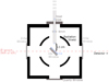 |
Fig. 1. Sketch of the cryocooler set-up. |
The gas mixtures were prepared in a 2 litre glass flask by using standard manometric techniques. The ratios of H2O to the O2 were adjusted by measuring the pressure inside the glass flask following the ideal gas law

whereas the number of H2O and O2 particles is set by the isotherm relation
where ni is the particle number, pi the partial pressure and Vi the partial volume of the gas i, in our case H2O and O2. The total pressure ptot is the sum of all partial pressures  and
and  .
.
The gas mixture composition used for each experiment is outlined in Table 1. Distilled water that had been degassed in a freeze-pump-thaw cycle three times, and oxygen with a purity of 99.999% were introduced in the cooling chamber under high vacuum with a base pressure of 10−6 mbar. The deposition time was varied starting with deposition times of 30 s, using a moderate deposition rate, and increasing the deposition time up to 3 min with fast depostion rate, so that thicknesses of 0.03 μm (∼100 MLs) up to 3 μm (∼10000 MLs), with an uncertainty of 20–30%, could be analysed. In the fourth column of Table 1, the water column density for thick ice reached after 1 min of deposition time for each ice mixture is listed; the derived water ice thickness and the oxygen column density are indicated in Cols. 5 and 6, respectively. We note that the latter has a high error for water rich ices due to limits in determing the area of the weak oxygen feature that is overlapped by the water bending vibration mode. Also, a comparison of NH2O and NO2 to estimate the real ice composition is difficult for oxygen rich ices due to monomer and dimer features in the water bands.
Gas mixture composition, expressed as partial pressure ratio, the water column density (NH2O), the water ice thickness dH2O and O2 column density (NO2) after a total deposition time of 1 min for thick ice for each experiment presented in this paper.
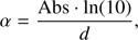
The thickness of the deposited ice has been calculated from the area of the three bands characteristic of the water ice spectral signature. First, the column density N has been estimated from the band area for the water component, following the relation
and for A using the band strength values from Hagen et al. (1981) and Gerakines et al. (1995). The factor ln(10) originates in the relation of the optical depth τ = Abs · ln(10) where Abs is the absorbance. τ is incorporated into the area. Then, the thickness d (cm) has been calculated assuming

where N is the column density (molecules cm−2), ρ the density (g cm−3), NA the Avogadro constant (molecules mol−1) and M the molecular mass (g mol−1). The total thickness has been estimated by considering the water to oxygen molecular ratio and scaling the thickness value accordingly. For this estimation we assumed that the ice molecular composition remains constant over the deposition time scale. There is no spectroscopic evidence which can prove that this assumption is correct, but assuming that the sticking coefficient is not varying significantly for the two components water and oxygen, we can estimate to produce a quite uniformly mixed ice. This is the general assumption used for this kind of experimental set-ups.
The cold KBr substrate is mounted with an angle of 45° with respect to the molecular beam direction. This configuration allows the deposition of the gas to take place simultaneously with the recording of the spectra. In the vacuum chamber, the molecules expand to a collisionless beam and the ice formed on the top of the substrate has a porous structure, with an expected density of approximately 0.8 g cm−3 (Dohnálek et al. 2003; Snels et al. 2011). The thickness values provided for these experiments have been scaled to the direction normal to the substrate surface, to correct for the 45° angle of the substrate with respect to the spectroscopic path.
The measurements in our experimental setup work in transmittance and thus we would take an ice deposition on both sides of the substrate into account. Nevertheless, we experimentally confirm that ice was deposited only on the side of the substrate that faces the steel pipe. We used the laser interference method to ensure that no significant amount of ice is deposited on the substrate face opposite to the gas inlet.
3. Results
3.1. O2 features in thin and thick ice samples
Figure 2 shows the whole observed spectrum for the different composition ratios after same deposition time. The figure clearly shows the H2O streching mode at 3280 cm−1, the H2O combination mode at 2200 cm−1, the H2O bending mode at 1660 cm−1 and the H2O libration mode at 760 cm−1. Moreover, the O2 feature can be found at 1551 cm−1. In spectra #2, #6, #7, and #8, features due to CO2 contamination are present at 2343 cm−1 and at 660 cm−1. The H2O:O2 = 2:1 spectrum shows the saturation of the stretching mode because of different deposition conditions compared to the other experiments.
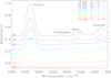 |
Fig. 2. Spectra of all H2O−O2 composition ratios for thick ice with same deposition time of 1 min each. The number of H2O monolayers here goes from 80 ML (thickness ≈ 0.03 μm) for H2O:O2 = 1:9 to 1900 ML (thickness ≈ 0.68 μm) for H2O:O2 = 9:1. The spectra for the different compositions are shifted in the absorbance scale for helping their visualization. The vertical red dashed line indicates the O2 band position at 1551 cm−1. |
In the thick ice layer regime (estimated thicknesses ranging between 1 and 3 μm) the oxygen feature is visible at all the investigated molecular ratio. Our limit cases are the mixture in excess of water (experiment #1) and the mixture in excess of oxygen (experiment #8). It is convenient to divide the analysis into two parts, one for the experiments from #1 to #4, and a second for the experiments from #5 to #8. In the first part, excess of water at different molecular ratios is investigated. In these experiments, the oxygen feature is overlapped to the bending vibration mode of water, making its detection increasingly difficult as the water becomes predominant in the molecular ratio (cf. Fig. 3). Nevertheless, even with a water to oxygen ratio of 9:1, the oxygen feature is still visible in our recorded spectrum, as it shown in Fig. 3.
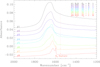 |
Fig. 3. Magnification of spectra of Fig. 2 around the O2 feature (marked by the vertical red dashed line) for all H2O−O2 mixtures for thick ice. |
For the thin ice, we conducted separate experiments in order to monitor the dependence of the O2 band position on the physical conditions of the thin ice. The spectrum of the thin H2O:O2 = 2:1 ice (thickness 0.022–0.053 μm) is shown enclosed around 1660 cm−1 in Fig. 4. Presenting even thinner ice, Fig. 5 shows the first three deposition steps (thickness 0.008–0.022 μm) in order to enhance the visibility of the O2 feature of which we see hints of the band at 1551 cm−1 also for the thinnest ice. The water bands assume the characteristic features of water trapped in a matrix, as can be observed from Ehrenfreund et al. (1996).
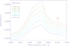 |
Fig. 4. Magnified spectra of H2O:O2 = 2:1 mixture around the O2 feature; the ice thicknesses is between 0.022 and 0.053 μm for thin ice. |
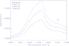 |
Fig. 5. Magnified spectra of H2O:O2 = 2:1 mixture around the O2 feature; the thicknesses is between 0.008 and 0.022 μm for thin ice. |
In the experiments in excess of oxygen, the O2 feature is progressively isolated from the water bending feature. Its spectral characteristics, though, are not varying significantly with the change in the H2O to O2 ratio, in terms of frequency shift and band profile. Therefore, these spectra offer the best conditions for the estimate of the O2 band strength. The band strength A is given as
where σ(̃v) is the cross-section (cm2) and τ(̃v) the optical depth for a given wavenumber ̃v (cm−1). Using
where Abs is the measured absorbance of the O2 feature, we get
We measured d̃v = 10 cm−1 and for O2 the column density N = 3.01 × 10²² mol cm−3 d. The derived band strengths for the different ice mixtures and a comparison with the values found by Ehrenfreund et al. (1992) can be found in Table 2.
Band strength (A) of O2 for the different ice compositions.
For comparable experiments, where the values of H2O/O2 presented in this work are equal to those presented by Ehrenfreund et al. (1992), the values of the band strength agree with a factor of approximately two. This difference is most likely due to the influence of CO and CO2 in the experiments conducted by Ehrenfreund et al. (1992), which enhance the oxygen band strength.
As the feature of solid O2 is present at 1551 cm−1, there exists the possibility for observable overtones in the NIR. While we don’t expect to see any O2 features near 3102 cm−1 (3.22 μm) due to the strong water signal, we looked for the next possible overtone at 4653 cm−1 (2.15 μm). Even, for the thick ice with 3 μm thickness, there is no O2 feature to be found near 4653 cm−1.
3.2. Dangling bonds
We note that in our experiments we dealt with a porous amorphous ice structure. For this reason, in the recorded spectra we observe the features assigned to the presence of the so-called dangling bonds, that is, features arising from the OH stretching vibration of water molecules that are not engaged in a intermolecular interaction with the ice bulk. Although the analysis of the spectral signature of the dangling bonds is not directly applicable to the comparison with astronomical observations, for which no detection is currently available, we believe that studying the way in which the presence of oxygen affects the features ascribed to the dangling bonds can provide useful information for future laboratory experiments. In Fig. 6 the spectral region of the dangling bonds for thick ice corresponding to the different H2O−O2 mixtures and the pure water is shown. The increasing steepness of the spectra towards 3500 cm−1 relate to the increasing ratio of H2O–O2 as the stretch feature of water rises in intensity with increasing water abundance. The positions of the dangling bond features can be found in Table 3.
 |
Fig. 6. Thick-ice absorption spectrum of H2O:O2 mixtures compared to pure water. To enable a better overview, similar to Fig. 2, the spectra of the different mixtures have been shifted. |
Gas mixture composition and position of the dangling bonds (with shoulder feature position where present) for each experiment presented in this paper.
Figure 6 shows a red shift of the dangling bonds peaks going from the pure water to the H2O:O2 = 2:1 mixture, from 3697 cm−1 (2.705 μm) and 3683 cm−1 (2.715 μm) to 3698 cm−1 (2.704 μm) and 3678 cm−1 (2.719 μm). The change in the spectroscopic feature of the dangling bonds for the water and oxygen ices with respect to pure water ice is in agreement with previous experiments performed by Palumbo et al. (2010), in which the effect on the profile of the dangling bond feature for an ice mixture of approximately 20% of oxygen in water is reported. Their study can be compared to our H2O:O2 = 4:1 mixture. For oxygen-rich ice mixtures, the peak shape and position is probably influenced by the presence of water monomers and dimers embedded in the oxygen matrix, as reported in Ehrenfreund et al. (1996).
4. Discussion
We decided to limit our study to the case of the molecular oxygen complexes with water and to extend the amount of molecular ratio explored going from ice mixtures in excess of water to excess of oxygen, in order to have a complete overview of the molecular oxygen signature in different astrophysical environments. Furthermore, for each experiment we have analysed the IR spectra in the thin and thick ice layer regimes, showing that the oxygen spectral signature does not exhibit different characteristics, in terms of band position and shape, with respect to the two approaches. The molecular vibration of O2 by itself is inactive in the infrared since the dipole moment doesn’t change upon molecular vibration. Nevertheless, the interaction with the water matrix breaks the electron symmetry and induce a small dipole moment, which allows for the detection in the IR region.
In the thin ice layer regime, in which the thicknesses of the ice layer (estimated for the water component) varys between 0.008 and 0.053 μm, the oxygen feature has been observed only in the most favourable case, that is, the H2O:O2 = 2:1 mixture (experiment #4). In this molecular ratio, the band strength of the oxygen feature is enhanced, as shown by Ehrenfreund et al. (1992), the instrumental detection limit in dealing with a low column density is overcome, and the observation of a low intensity band is possible. For even thinner ices however, we don’t expect the shape and position of the O2 feature to change much, but the detection of O2 depends on the total column density, so in the end it depends on the ice thickness as well as dust number density. In the remaining cases the low intensity of the band signal did not allow for a detection. The frequency position measured in the experiment #4 is 1551 cm−1 (6.45 μm). In order to increase the S/N for the thin H2O:O2 = 2:1 ice, the recording of the spectra was performed with a higher number of recorded cycles (2048 record cycles; for comparison: 1184 record cycles for thick ice). That way, the noise was reduced in order to obtain a S/N ≲3 even for the thinnest ice.
In addition, we compared the dangling bond features of pure water with that of the H2O:O2 = 9:1 mixtures. As already observed by Palumbo et al. (2010), the profile of the dangling bond feature depends on the presence of other species mixedin with water ice. The presence of oxygen affects the dangling bonds profile in term of intensity and shape. Their profile may be related to the microstructure of the deposited ice. As can be observed from Fig. 6, the H2O:O2 ratio in the ice is affecting significantly the spectral characteristic of the water dangling bonds. Going from the water rich to oxygen rich mixtures, we observe a progressive change in the relative intensity of the two main features and a shift in their position. For oxygen rich mixtures, we observe a predominant sharper feature at lower frequencies, while the water rich mixtures exhibit a smoother profile and similar relative intensities of the two components. The mixture with a similar water to oxygen ratio shows a profile which is in between the extremes. From this consideration we can relate the shape of the dangling bonds bands with the molecular composition of the bulk ice, allowing an identification of the enrichment of the ice in one or the other species. However, a detailed analysis of the effect of the structure of the ice on the dangling bond characteristic is outside the scope of this work.
Figure 7 shows the behaviour of the O2 feature upon heating. Observed O2 features started to vanish when the probes were heated to 35 K. At this temperature, the O2 molecules trapped on the amorphous water ice matrix start to evaporate (cf. Bar-Nun et al. 1987). At a temperature of 50 K, the O2 features were completely absent. Above this temperature the O2 is not trapped by the porous amorphous solid water any more and the O2 is desorbed from the deposited ice. This observation is consistent with the experiments conducted by Ayotte et al. (2001).
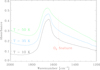 |
Fig. 7. Behaviour of the O2 feature (marked by the vertical dashed line) for H2O:O2 = 2:1 while heating the ice from 10 K to 50 K. |
5. Astrophysical implications
Our experimental approach intends to explore astrophysical scenarios. The experiments dedicated to the thin ice layer regime (number of monolayers < 150; counted using the thickness and density of the ice) simulate the conditions in the dense interstellar medium more adequately (Öberg 2016), while the experiments in the thick layer regime attempt to extend the physical conditions relative to the centre of pre-stellar cores as well as in the midplane of protoplanetary disks, where pebbles and icy bodies precursors of comets and planetesimals with ice thicknesses >200 ML form (e.g. Bieler et al. 2015). There is a lack of observational data proving the presence of molecular oxygen in ISM ice, while O2 has been recently detected in the coma of the comet 67P/Churyumov-Gerasimenko (Bieler et al. 2015; Mousis et al. 2016).
Our experimental data show that the detection of the O2 feature in thin ices is much more difficult compared to the thick ones, and the only molecular composition allowing the laboratory detection is the H2O:O2 = 2:1, which is unrealistic for the ISM ice composition. However, predictions by astrochemical models for pre-stellar cores, such as L1544, indicate that the icy mantles can reach thicknesses close to the thick ice regime in these experiments (e.g. Vasyunin et al. 2017). On the other hand, the mixture with a molecular ratio H2O:O2 = 9:1 will account for a realistic proportion like it was observed in the cometary coma of 67P/Churyumov-Gerasimenko with a mean value of 3.80 ± 0.85%.
5.1. Chemical modelling
We studied which ice structure and composition is predicted by current astrochemical models, and how it is related to the observational data on O2:H2O ratio and ice thickness. For this purpose, we used results from Vasyunin et al. (2017). Briefly, this is a three-phase (gas-reactive ice surface – (less) reactive ice bulk) time-dependent astrochemical model that includes an extensive set of gas-phase and grain-surface chemistry. In Vasyunin et al. (2017), the model has been successfully applied to the explanation of observed distribution of complex organic molecules (COMs) in the prototypical pre-stellar core L1544. The authors find that the best agreement between the model and the observed data is reached after 1.6 × 10⁵ years of chemical evolution of a static cloud with physical structure similar to one reproduced for L1544. The model also reproduced the enchanced abundances of COMs at the so-called methanol peak located ∼4000 AU (∼0.015 pc) away from the centre of the core (the peak of the dust emission), as observed by Bizzocchi et al. (2014).
At the time of maximum O2/H2O abundance, the modelled ice thickness is 70 monolayers, but it is growing with time, and stabilizes at the methanol peak at 200 monolayers after 105 years of evolution, as shown in Fig. 8. As such, we believe that modelling results are in rough agreement with observed values for O2/H2O in the coma of 67P/Churyumov-Gerasimenko comet. Also, the modelling suggests that icy mantles in pre-stellar cores such as L1544 are relatively thick, and may reach several hundreds of monolayers. Finally, it is interesting to note that while the model by Vasyunin et al. (2017) predicts gas-phase O2 abundance, at the time of the best agreement between the model and observed values of COMs, to be at least an order of magnitue lower than that of CO, the O2 gas-phase abundance is still overestimated by an order of magnitude in comparison to observed upper limits in other environments (e.g. Goldsmith et al. 2000). The gasphase O2 abundance in the model by Vasyunin et al. (2017) is mainly controlled by the reactive desorption mechanism, whose efficiency under various conditions is currently a matter of debate (see e.g. Minissale et al. 2016; Chuang et al. 2018; He et al. 2017; Oba et al. 2018). Thus, gas-phase abundance of O2 will be the subject of further theoretical and experimental studies.
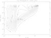 |
Fig. 8. Model ice thickness (in monolayers) vs. time in L1544. The “methanol peak” is located 4000 AU away from the core centre. |
5.2. Astronomical observability
Using absorbance and thickness data obtained in our experiments, we were able to calculate the absorption coefficient
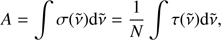
for the different mixture ratios of O2/H2O. α as a function of the O2/H2O ratio can be found in Fig. 9. The absorption coefficients for water are in good agreement with the derived values from Warren & Brandt (2008), considering a discrepancy in sample temperature, while we have no possibility to compare the calculated absorption coefficient for O2 with the literature. In order to calculate α for all O2–H2O ratios, the data were fit using two different methods for statistical comparison. The first method creates the fit by minimizing the χ2-error statistics. The second method uses the least absolute deviation method that minimizes the sum of absolute errors.
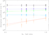 |
Fig. 9. Absorption coefficients of the 3280 cm−1 (black), 2200 cm−1 (light blue), 1660 cm−1 (green), 760 cm−1 (dark blue) water and 1551 cm−1 (red) O2 bands for the different mixture ratios of O2 and H2O. The data were fit using the (a) minimizing χ2-error statistics (bright coloured fits) and (b) “robust” least absolute deviation method (dark coloured fits). |
The calculated values were then used to derive the optical depth and the transmittance of L1544 using the model by Vasyunin et al. (2017) introduced in Sect. 5.1 (cf. Fig. 10). The transmittance of an area with a constant absorption coefficient can be calculated with
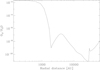 |
Fig. 10. Calculated O2/H2O of L1544 as a function of the radial distance for t = 1.6 × 10⁵ yr. |
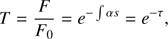
where F0 is the initial flux density received from the medium, F is the flux density transmitted by the medium, s is the size of the area with a certain absorption coefficient α. For our calculations, we divide the modelled cloud into subpaths sn of constant absorption coefficients and obtain

Following this, we get the total transmittance

The optical depth and transmittance was computed only for the inner part of our modelled L1544 where O2/H2O is > 10−6. The derived optical depth and transmittance for the different H2O and O2 can be found in Table 4.
Optical depth and transmittance of the modelled L1544 in the area with O2/H2O > 10−6.
Directly comparing the overlapping H2O 1660 cm−1 and O2 1551 cm−1 bands we get a transmittance ratio of 0.946 for fitting method a) and b). The predicted transmittance of the O2 band is then ≈5.4% of the water band transmittance at 1660 cm−1. In order to check the observability of this feature with the James Webb Space Telescope (JWST) the time calculator facility has been employed. For the prestellar core L1544, we calculated the time needed to detect the O2 line at a 3σ level for the MIRI instrument in the Channel 1 (short) configuration and found that this requires more than 100 h with JWST, meaning it is not feasible. This estimate is, however, conservative, as we expect, based on the experiments by Ehrenfreund et al. (1992), that the O2 feature becomes stronger when ice mixtures are considered. We will quantify this in a future paper, where we will present the spectroscopic signatures of an ice mixture similar to the one predicted by Vasyunin et al. (2017).
6. Conclusions
This paper presents spectral features of solid molecular oxygen enclosed in a water matrix. The analysis is compared to previous studies reported by Ehrenfreund et al. (1992) and Palumbo et al. (2010), and extended to further molecular ratios and ice thicknesses, as motivated by the recent detection of O2 in the comet 67P/Churyumov-Gerasimenko. In particular, we have explored the possibility of detecting O2 in solid form towards pre-stellar cores for which gas-grain chemical model predictions were available.
In our experiments, O2 is found at 1551 cm−1 for thick ice. Also, we find evidence for the O2 band at that position even for our thinnest ice. Because of their more heterogeneous composition, interstellar ices may, however, show the O2 features around these values. The porous amorphous nature of the ice mixture produces the dangling bonds near the stretching mode of water. However, while their position and intensity depends on the ratio of H2O and O2, the lack of detection in space hint to the conclusion that the ice there is compact and not porous (e.g. Palumbo 2005). The O2 feature can only be seen for temperatures ≤35 K.
The behaviour of the dangling bonds in dependence of the ice mixture composition has been discussed. The O2:H2O ratio not only has an effect on the intensity of the features but also on their position and shape. This is especially so for mixtures with an excess of O2 that show a shoulder feature or even a second maximum near the two main bands.
The three-phase time-dependent astrochemical model of the pre-stellar core L1544, as introduced by Vasyunin et al. (2017) predicts thick ice (≈200 ML) and O2/H2O fractions close to those measured towards the comet 67P. Using JWST, it is not feasible to detect O2 in solid phase via measuring the transmission ratio of L1544 using the MIRI instrument. New estimates for the O2 detection in mixed ices with JWST, however, will be done in a future paper.
Acknowledgments
The authors thank the anonymous referee, who greatly helped us to enhance the clarity of the paper. We thank Christian Deysenroth for the very valuable contribution in the designing and mechanical work of the experimental setup. We are also grateful to Miwa Goto, Wing-Fai Thi, and Seyit Hocuk for fruitful discussion. The work of Birgitta Müller was supported by the IMPRS on Astrophysics at the Ludwig-Maximilians University, as well as by the funding the IMPRS receives from the Max-Planck Society. The work of Anton Vasyunin is supported by the Russian Science Foundation via the Project No. 18-12-00351.
References
- Ayotte, P., Smith, R. S., Stevenson, K. P., et al. 2001, J. Geophys. Res.: Planets, 106, 33387 [NASA ADS] [CrossRef] [Google Scholar]
- Bar-Nun, A., Dror, J., Kochavi, E., & Laufer, D. 1987, Phys. Rev. B, 35, 2427 [NASA ADS] [CrossRef] [Google Scholar]
- Bergin, E. A., Melnick, G. J., Stauffer, J. R., et al. 2000, ApJ, 539, L129 [NASA ADS] [CrossRef] [Google Scholar]
- Bieler, A., Altwegg, K., Balsiger, H., et al. 2015, Nature, 526, 678 [Google Scholar]
- Bizzocchi, L., Caselli, P., Spezzano, S., & Leonardo, E. 2014, A&A, 569, A27 [NASA ADS] [CrossRef] [EDP Sciences] [Google Scholar]
- Boogert, A., Gerakines, P., & Whittet, D. 2015, ARA&A, 53, 541 [Google Scholar]
- Breukers, R. J. L. H. 1991, PhD Thesis, University of Leiden, The Netherlands [Google Scholar]
- Carty, D., Goddard, A., Köhler, S. P. K., Sims, I. R., & Smith, I. W. M. 2006, J. Phys. Chem. A, 110, 3101 [CrossRef] [PubMed] [Google Scholar]
- Chuang, K.-J., Fedoseev, G., Qasim, D., et al. 2018, ApJ, 853, 102 [NASA ADS] [CrossRef] [Google Scholar]
- Cuppen, H. M., & Herbst, E. 2007, ApJ, 668, 294 [Google Scholar]
- Davidsson, J., & Stenholm, L. G. 1990, A&A, 230, 504 [NASA ADS] [Google Scholar]
- Dohnálek, Z., Kimmel, G. A., Ayotte, P., Smith, R. S., & Kay, B. D. 2003, J. Chem. Phys., 118, 364 [NASA ADS] [CrossRef] [Google Scholar]
- Dulieu, F., Amiaud, L., Congiu, E., et al. 2010, A&A, 512, A30 [NASA ADS] [CrossRef] [EDP Sciences] [Google Scholar]
- Ehrenfreund, P., & van Dishoeck, E. 1998, AdSpR, 21, 15 [NASA ADS] [CrossRef] [Google Scholar]
- Ehrenfreund, P., Breukers, R., d’Hendecourt, L., & Greenberg, J. 1992, A&A, 260, 431 [NASA ADS] [Google Scholar]
- Ehrenfreund, P., Gerakines, P. A., Schutte, W. A., van Hemert, M. C., & van Dishoeck, E. F. 1996, A&A, 312, 263 [NASA ADS] [Google Scholar]
- Gerakines, P. A., Schutte, W. A., Greenberg, J. M., & van Dishoeck, E. F. 1995, A&A, 296, 810 [NASA ADS] [Google Scholar]
- Goldsmith, P. F., Melnick, G. J., Bergin, E. A., et al. 2000, ApJ, 539, L123 [NASA ADS] [CrossRef] [Google Scholar]
- Goldsmith, P. F., Liseau, R., Bell, T. A., et al. 2011, ApJ, 737, 96 [Google Scholar]
- Hagen, W., Tielens, A. G. G. M., & Greenberg, J. M. 1981, Chem. Phys., 56, 367 [NASA ADS] [CrossRef] [Google Scholar]
- Hama, T., & Watanabe, N. 2013, Chem. Rev., 113, 8783 [CrossRef] [Google Scholar]
- He, J., Emtiaz, S. M., & Vidali, G. 2017, ApJ, 851, 104 [NASA ADS] [CrossRef] [Google Scholar]
- Herbst, E., & Millar, T. J. 2008, The Chemistry of Cold Interstellar Cloud Cores, ed. I. W. M. Smith (Imperial College Press), 1 [Google Scholar]
- Ioppolo, S., Cuppen, H. M., Romanzin, C., van Dishoeck, E. F., & Linnartz, H. 2008, ApJ, 686, 1474 [NASA ADS] [CrossRef] [Google Scholar]
- Ioppolo, S., van Boheemen, Y., Cuppen, H. M., van Dishoeck, E. F., & Linnartz, H. 2011, MNRAS, 413, 2281 [NASA ADS] [CrossRef] [Google Scholar]
- Jing, D., He, J., Brucato, J. R., et al. 2012, ApJ, 756, 98 [NASA ADS] [CrossRef] [Google Scholar]
- Keeney, B. A., Stern, S. A., A’Hearn, M. F., et al. 2017, MNRAS, 469, S158 [CrossRef] [Google Scholar]
- Larsson, B., Liseau, R., Pagani, L., et al. 2007, A&A, 466, 999 [Google Scholar]
- Liseau, R., Goldsmith, P. F., Larsson, B., et al. 2012, A&A, 541, A73 [NASA ADS] [CrossRef] [EDP Sciences] [Google Scholar]
- Minissale, M., Dulieu, F., Cazaux, S., & Hocuk, S. 2016, A&A, 585, A24 [NASA ADS] [CrossRef] [EDP Sciences] [Google Scholar]
- Miyauchi, N., Hidaka, H., Chigai, T., et al. 2008, Chem. Phys. Lett., 456, 27 [NASA ADS] [CrossRef] [Google Scholar]
- Mokrane, H., Chaabouni, H., Accolla, M., et al. 2009, ApJ, 705, L195 [NASA ADS] [CrossRef] [Google Scholar]
- Mousavipour, S. H., & Saheb, V. 2007, Bull. Chem. Soc. Jpn., 80, 1901 [CrossRef] [Google Scholar]
- Mousis, O., Ronnet, T., Brugger, B., et al. 2016, ApJ, 823, L41 [NASA ADS] [CrossRef] [Google Scholar]
- Oba, Y., Miyauchi, N., Hidaka, H., et al. 2009, ApJ, 701, 464 [NASA ADS] [CrossRef] [Google Scholar]
- Oba, Y., Watanabe, N., Hama, T., et al. 2012, ApJ, 749, 67 [NASA ADS] [CrossRef] [Google Scholar]
- Oba, Y., Tomaru, T., Lamberts, T., Kouchi, A., & Watanabe, N. 2018, Nat. Astron., 2, 228 [NASA ADS] [CrossRef] [Google Scholar]
- Öberg, K. I. 2016, Chem. Rev., 116, 9631 [Google Scholar]
- Palumbo, M. E. 2005, J. Phys: Conf. Ser., 6, 211 [NASA ADS] [CrossRef] [Google Scholar]
- Palumbo, M. E., Baratta, G. A., Leto, G., & Strazzulla, G. 2010, J. Mol. Struct., 972, 64 [NASA ADS] [CrossRef] [Google Scholar]
- Romanzin, C., Ioppolo, S., Cuppen, H. M., van Dishoeck, E. F., & Linnartz, H. 2011, J. Chem. Phys., 134, 084504 [NASA ADS] [CrossRef] [Google Scholar]
- Snels, M., Horká-Zelenková, V., Hollenstein, H., & Quack, M. 2011, Handbook of High-resolution Spectroscopy (John Wiley & Sons, Ltd.), 2, 1021 [Google Scholar]
- Taquet, V., Furuya, K., Walsh, C., & van Dishoeck, E. F. 2016, MNRAS, 462, 99 [NASA ADS] [CrossRef] [Google Scholar]
- Tielens, A. G. G. M., & Hagen, W. 1982, A&A, 114, 245 [Google Scholar]
- Vandenbussche, B., Ehrenfreund, P., Boogert, A., et al. 1999, A&A, 346, L57 [NASA ADS] [Google Scholar]
- Vasyunin, A. I., Caselli, P., Dulieu, F., & Jiménez-Serra, I. 2017, ApJ, 842, 33 [Google Scholar]
- Viti, S., Roueff, E., Hartquist, T. W., des Forêts, G. P., & Williams, D. A. 2001, A&A, 370, 557 [NASA ADS] [CrossRef] [EDP Sciences] [Google Scholar]
- Warren, S. G., & Brandt, R. E. 2008, J. Geophys. Res., 113, D14220 [Google Scholar]
- Woodall, J., Agúndez, M., Markwick-Kemper, A. J., & Millar, T. J. 2007, A&A, 466, 1197 [NASA ADS] [CrossRef] [EDP Sciences] [Google Scholar]
All Tables
Gas mixture composition, expressed as partial pressure ratio, the water column density (NH2O), the water ice thickness dH2O and O2 column density (NO2) after a total deposition time of 1 min for thick ice for each experiment presented in this paper.
Gas mixture composition and position of the dangling bonds (with shoulder feature position where present) for each experiment presented in this paper.
Optical depth and transmittance of the modelled L1544 in the area with O2/H2O > 10−6.
All Figures
|
Fig. 1. Sketch of the cryocooler set-up. |
| In the text | |
|
Fig. 2. Spectra of all H2O−O2 composition ratios for thick ice with same deposition time of 1 min each. The number of H2O monolayers here goes from 80 ML (thickness ≈ 0.03 μm) for H2O:O2 = 1:9 to 1900 ML (thickness ≈ 0.68 μm) for H2O:O2 = 9:1. The spectra for the different compositions are shifted in the absorbance scale for helping their visualization. The vertical red dashed line indicates the O2 band position at 1551 cm−1. |
| In the text | |
|
Fig. 3. Magnification of spectra of Fig. 2 around the O2 feature (marked by the vertical red dashed line) for all H2O−O2 mixtures for thick ice. |
| In the text | |
|
Fig. 4. Magnified spectra of H2O:O2 = 2:1 mixture around the O2 feature; the ice thicknesses is between 0.022 and 0.053 μm for thin ice. |
| In the text | |
|
Fig. 5. Magnified spectra of H2O:O2 = 2:1 mixture around the O2 feature; the thicknesses is between 0.008 and 0.022 μm for thin ice. |
| In the text | |
|
Fig. 6. Thick-ice absorption spectrum of H2O:O2 mixtures compared to pure water. To enable a better overview, similar to Fig. 2, the spectra of the different mixtures have been shifted. |
| In the text | |
|
Fig. 7. Behaviour of the O2 feature (marked by the vertical dashed line) for H2O:O2 = 2:1 while heating the ice from 10 K to 50 K. |
| In the text | |
|
Fig. 8. Model ice thickness (in monolayers) vs. time in L1544. The “methanol peak” is located 4000 AU away from the core centre. |
| In the text | |
|
Fig. 9. Absorption coefficients of the 3280 cm−1 (black), 2200 cm−1 (light blue), 1660 cm−1 (green), 760 cm−1 (dark blue) water and 1551 cm−1 (red) O2 bands for the different mixture ratios of O2 and H2O. The data were fit using the (a) minimizing χ2-error statistics (bright coloured fits) and (b) “robust” least absolute deviation method (dark coloured fits). |
| In the text | |
|
Fig. 10. Calculated O2/H2O of L1544 as a function of the radial distance for t = 1.6 × 10⁵ yr. |
| In the text | |
Current usage metrics show cumulative count of Article Views (full-text article views including HTML views, PDF and ePub downloads, according to the available data) and Abstracts Views on Vision4Press platform.
Data correspond to usage on the plateform after 2015. The current usage metrics is available 48-96 hours after online publication and is updated daily on week days.
Initial download of the metrics may take a while.