| Issue |
A&A
Volume 608, December 2017
|
|
|---|---|---|
| Article Number | A115 | |
| Number of page(s) | 10 | |
| Section | Extragalactic astronomy | |
| DOI | https://doi.org/10.1051/0004-6361/201731853 | |
| Published online | 13 December 2017 | |
Chandra imaging of the ~kpc extended outflow in 1H 0419-577
1 Department of Astronomy, University of Geneva, 16 Ch. d’ Ecogia, 1290 Versoix, Switzerland
e-mail: laura.digesu@unige.ch
2 SRON Netherlands Institute for Space Research, Sorbonnelaan 2, 3584 CA Utrecht, The Netherlands
3 Osservatorio Astronomico di Roma (INAF), via Frascati 33, 00040 Monteporzio Catone (Roma), Italy
4 Leiden Observatory, Leiden University, PO Box 9513, 2300 RA Leiden, The Netherlands
Received: 29 August 2017
Accepted: 2 October 2017
The Seyfert 1 galaxy 1H 0419-577 hosts a ~kpc extended outflow that is evident in the [O iii] image and that is also detected as a warm absorber in the UV/X-ray spectrum. Here, we analyze a ~30 ks Chandra-ACIS X-ray image, with the aim of resolving the diffuse extranuclear X-ray emission and of investigating its relationship with the galactic outflow. Thanks to its sub-arcsecond spatial resolution, Chandra resolves the circumnuclear X-ray emission, which extends up to a projected distance of at least ~16 kpc from the center. The morphology of the diffuse X-ray emission is spherically symmetrical. We could not recover a morphological resemblance between the soft X-ray emission and the ionization bicone that is traced by the [O iii] outflow. Our spectral analysis indicates that one of the possible explanations for the extended emission is thermal emission from a low-density (nH ~ 10-3 cm-3) hot plasma (Te ~ 0.22 keV). If this is the case, we may be witnessing the cooling of a shock-heated wind bubble. In this scenario, the [O iii] emission line and the X-ray/UV absorption lines may trace cooler clumps that are entrained in the hot outflow. Alternatively, the extended emission could be to due to a blend of emission lines from a photoionized gas component having a hydrogen column density of NH ~ 2.1 × 1022 cm-2 and an ionization parameter of log ξ ~ 1.3. Because the source is viewed almost edge-on we argue that the photoionized gas nebula must be distributed mostly along the polar directions, outside our line of sight. In this geometry, the X-ray/UV warm absorber must trace a different gas component, physically disconnected from the emitting gas, and located closer to the equatorial plane.
Key words: quasars: general / quasars: emission lines / quasars: absorption lines / galaxies: individual: 1H 0419-577 / X-rays: galaxies
© ESO, 2017
1. Introduction
The X-ray emission from type-1 active galactic nuclei (AGN) is dominated by the bright nucleus. However, besides providing a diagnostic of the physics in the vicinity of the black hole, the X-ray domain offers the possibility of probing the extranuclear AGN environment. For instance, with the advent of the Chandra satellite, X-ray imaging at sub-arcsecond spatial resolution became possible, thereby allowing detailed studies of the circumnuclear gaseous environment in a handful of nearby Seyferts.
Observation log.
Extranuclear X-ray emission has been detected with Chandra up to distances of the order of a few tenths of a kpc both in Seyfert 2 (e.g., Circinus, Smith & Wilson 2001; NGC 1068, Young et al. 2001; NGC 4388, Iwasawa et al. 2003) and in Seyfert 1 galaxies (e.g., NGC 1365, Wang et al. 2009; NGC 4151, Wang et al. 2011). In type-2 AGN it is often observed that the X-ray morphology resembles the ionization bicone (Pogge 1988), which is traced for instance by the [O iii] narrow line (NL). The morphological correspondence points to an origin in the same medium photoionized by the central AGN which has been, in a few cases, confirmed using photoionization analysis techniques in combination with high-resolution X-ray spectroscopy (Bianchi et al. 2006; Gonzalez-Martin et al. 2010). However, hot, collisionally ionized plasma, may, in some cases, coexist in the ionization cone with the cooler photoionized plasma and act as a confining medium for the photoionized clouds (e.g., NGC 1365, Wang et al. 2009).
It has also been proposed (Guainazzi & Bianchi 2007) that the emitting gas in the NL ionization cone is the counterpart in emission of the so-called warm absorbers (WA) that are instead observed in high-resolution X-ray/UV spectra of nearby Seyfert-1 (Crenshaw et al. 2003; Piconcelli et al. 2005). These WA highlight gentle outflows of photoionized gas (v ~ 100–1000 km s-1, McKernan et al. 2007) that may be located at distances of the order 0.01–100 pc (Crenshaw & Kraemer 2012) from the nucleus. Spatially resolved spectroscopic studies of the [O iii] emission line in nearby Seyferts show indeed that the kinetics of the gas in the ionization cone is dominated by a radial outflow (Fischer et al. 2013), which is another hint to a possible connection. However, proving a firm connection would require an accurate knowledge of the physical parameters (the hydrogen column densityNHand the ionization parameter ξ) and of both the emitting and the absorbing gas, which is rarely the case. Indeed, parameterizing the NL emitting gas requires lengthy photoionization calculations, that have been carried out only in a few cases so far (e.g., Nucita et al. 2010; Di Gesu et al. 2013; Whewell et al. 2015, 2016).
The estimations (e.g., Detmers et al. 2009; Ebrero et al. 2016; Behar et al. 2017) of the kinetic luminosity (Lkin) carried by the WA in Seyfert-type AGN indicates that they are not energetically significant for possible AGN feedback (Di Matteo et al. 2005; Hopkins & Elvis 2010). Galactic molecular winds, that are often extended on ~kpc scales, and that can be either AGN (e.g., Mrk 231, Feruglio et al. 2015) or starburst driven (see e.g., Veilleux et al. 2005, for a review), may be a more effective feedback agent because they may be able to displace a sizeable amount of cold gas, thereby leading to starvation of the star-formation (SF) in the galaxy. High spatial-resolution X-ray imaging is also a way to test if and how some feedback is being exerted on the galactic medium, because the mechanical shock associated with a large-scale outflow is a viable mechanism to heat the gas up to X-ray energies. Diffuse hot gas, consistent with being shock-heated by a starburst wind, has been detected on a 5 kpc scale in the Chandra image of NGC 6240 (Wang et al. 2014). In another work, Wang et al. (2010) discovered diffuse soft X-ray emission in the central ~2 kpc of NGC 4151, which can be ascribed to a thermally emitting gas, mechanically heated by an AGN outflow. A 65 × 50 kpc X-ray nebula was also detected in a long-exposed Chandra-ACIS image of Mrk 231 (Veilleux et al. 2014), which is considered the prototypical case of galactic-scale, quasar-driven outflow involving both a neutral and a mildly ionized phase of the medium (Rupke & Veilleux 2013). In that case, the lack of cool soft X-ray emitting gas in a region corresponding to a large column of outflowing neutral gas can be interpreted as evidence of shock heating due to the massive quasar outflow.
The bright quasar known as 1H 0419-577 (or IRAS F04250-5718) is spectrally classified as Seyfert 1.5 (Véron-Cetty & Véron 2006), and is a radio-quiet AGN located at a redshift of 0.104.
It was previously found that, at X-ray energies smaller than ~2 keV, this source displays a highly variable soft-excess (Singh et al. 1985), with frequent transitions between low and high flux states on timescales of months/years (Guainazzi et al. 1998). The quest of understanding the origin of this variability motivated a rich, multi-epoch X-ray spectral coverage that includes six XMM-Newton (Page et al. 2002; Pounds et al. 2004a,b) and two Suzaku observations (Turner et al. 2009; Pal & Dewangan 2013). In Di Gesu et al. (2014), we fitted the deep (97 ks) XMM-Newton EPIC-pn spectrum together with the optical/UV flux data points with a Comptonization model. In this model, the optical/UV disk photons are up-scattered to X-ray energies by two intervening layers of plasma, with T ~ 100 keV and T ~ 0.5 keV, respectively. With the addition of an intervening neutral absorber, variable in column density, our model is able to explain also the historical optical-to-X-ray spectral variability of the source.
This long XMM-Newton observation was taken simultaneously with a HST-COS observation in the UV, with the aim of detecting and characterizing a photoionized WA. In the high-quality RGS spectrum we detected the absorption lines (e.g., O iv–O vi) of a lowly ionized WA (log NH ~ 19.9 cm-2, log ξ ~ 0.03 erg cm s-1), which is consistent with being one and the same as the UV absorber. Combining X-ray and UV diagnostics, we estimated that the absorption lines arise in a galactic wind, located at a distance of at least ~4 kpc from the nucleus. Since then, the estimated location was confirmed using Integral Field Unit (IFU) optical spectroscopy (at the GEMINI telescope Liu et al. 2015). The velocity-resolved [O iii] map shows indeed a biconical outflow extending up at to at least ~3 kpc from center. The outflow axis is tilted at ~20°with respect to the galactic disk and the opening angle of each cone is ~70°.
Extended, circumnuclear X-ray emission from 1H 0419-577 was noticed for the first time in the ROSAT HRI image. After a careful recalibration of the HRI PSF, which was carried out using a sample of bright point-like sources1, Predehl & Prieto (2001) concluded that “the Seyfert 1 galaxy 1H 0419-577 seems to be really extended”.
Here, we present the results of a Chandra-ACIS observation of 1H 0419-577, that we performed with the aim of resolving the extended X-ray emission in this source and of investigating its possible connection with the galactic outflow. The plan of the paper is as follows. In Sect. 2 we describe the data preparation while in Sects. 3 and 4 we present the imaging and the spectral analysis, respectively. Finally, in Sect. 5 we discuss our results and in Sect. 6 we present our conclusions.
For the present analysis, we considered a flat universe, with H0 = 70 km s-1 Mpc-1, Ωm = 0.3, ΩΛ = 0.7. With these cosmological parameters 1′′ corresponds to 1.9 kpc at the redshift of 1H 0419-577. The C-statistics (Cash 1979) is used throughout the paper and errors are quoted for ΔC = 2.7. In all the spectral models presented in the following we consider the Galactic hydrogen column density from Kalberla et al. (2005,NH = 1.26 × 1020 cm-2.
2. Observations and data preparation
2.1. Data reduction
In Table 1 we outline the summary of our Chandra observation of 1H 0419-577 which was carried out in May 2016. The total observing time of ~30 ks was split into two shorter exposures of ~8 and ~20 ks, respectively. Our observation was performed with only the back-illuminated S3 chip of the ACIS detector on. We chose the 1/8 subarray configuration, which reduces the frame time to ~0.4 s, to minimize a possible nuclear pile-up.
Throughout the paper, we compare 1H 0419-577 with PKS 2126-158, a bright blazar located at z = 3.26, which can be considered a prototypical point-like source. We retrieved the Chandra data of PKS 2126-158, that were taken with the same detector configuration as our observation, from the public Chandra archive (Obs ID: 376).
We performed the data analysis using the latest version of the software CIAO (v. 4.9) in combination with the most up-to-date calibration database CALDB 4.7.3. We reduced all the Chandra data using the chandra_repro script and we removed the ACIS readout-streak from the calibrated event-files. For 1H 0419-577, we created a merged, ~28 ks exposed event-file. For this purpose, we first cross-matched the WCS coordinates of the two event files using those of the longest one as reference. We ran the wavdetect task for source detection for both the event files, and we input the two obtained source lists in the CIAO task reproject_aspect. We set the task to apply the WCS correction to the 8 ks event-file, which minimizes the differences between the two source lists. The source centroid found by wavdetect is 4:26:00.7, −57:12:02, which is consistent with the nominal coordinates of 1H 0419-577. We use these coordinates in the remainder of the analysis. Hence, we merged the corrected 8 ks event-file and the 20 ks event-file using the CIAO tool reproject_obs.
We checked the event-files for possible photon pile-up. The CIAO task pileup_map creates an image in counts per ACIS frame, which can be used to estimate the pile-up fraction. The map shows that the nucleus of 1H-0419-577 is piled-up at a level of ~10% in a 3 × 3 pixels island around the nucleus. We consider this level of pile-up acceptable for our analysis and we comment on it below. Finally, we note that in the observation of PKS 2126-128, that we use as a comparison, the pile-up fraction is the same.
 |
Fig. 1 Chandra-ACIS images of 1H 0419-577 (top left) and of the point-like source PKS 2126-158 (top right) in the 0.2–1.0 keV band. As a visual aid, we also show the color bar of these two images at the bottom. For comparison, we show in both the panels a circle with the radius of the core of the Chandra PSF. Bottom left: same as first panel, smoothed using a Gaussian kernel of 3 pixels. The regions that we used for spectral extraction are overlaid. We also mark the direction from which we removed the ACIS readout streak (dashed line) and the location of possible extended filaments around the source. Bottom right: false-color image obtained using the PSF-deconvolved 0.2–0.5, 0.5–2.0, and 2.0–7.0 keV band images as red, green, and blue, respectively. |
2.2. PSF simulations
In order to disentangle possible extended emission from the bright point-like nucleus, accurate modeling of the instrumental point spread function (PSF) is needed. We used the Chandra HRMA ray tracer (ChaRT) to simulate a Chandra observation of a point-like source having the same spectrum as the nucleus of 1H 0419-577. We extracted the nuclear spectrum in a circular region having a radius of 2′′ from which we excluded a 3 × 3 pixels box including the piled-up area. A phenomenological model, comprising a power-law plus a blackbody provides an adequate fit spectrum of the nucleus extracted in this region. Besides the model spectrum of the nucleus, we input in ChaRT the same satellite configuration of our observation and the aspect-solution of the 20 ks event file. We treated the ChaRT outputs with the CIAO script simulate_psf, which uses MARX (v. 5.3.0) to project rays onto the detector and to create the PSF pseudo event-file. Starting from that, we created images and surface-brightness profiles of the PSF in the 0.2–1.0 keV and 1.0–7.0 keV energy bands. We used the PSF images (see below) for the PSF deconvolution of the source images that we performed using the Lucy-Richardson (Lucy 1974) method as implemented in the arestore task in CIAO.
2.3. Spectra preparation
We extracted all the spectra and spectral response matrices using the script specextract, which is provided in CIAO. We took the spectrum of the nucleus from a circular region with a radius of 2′′. Conversely, we extracted the spectrum of the extended emission in an annulus centered on the same coordinates and with an inner and an outer radius of 2′′ and 8′′, respectively. As a comparison (see below), we also extracted the spectra of PKS 2126-128 in the same regions. In all cases, we took the spectrum of the background from an exterior annulus 3′′ wide. For 1H 0419-577, we extracted the spectra from each individual observation as recommended in the CIAO guidelines. Hence, in all cases, we co-added the spectra in a single 28 ks exposed spectrum. We summed the spectra using the FTOOL mathpha and averaged the ancillary response files with addarf.
All the spectral analysis outlined in Sect. 4 was performed using the latest version of the SPEX program (v.3.03.00). The C-statistics, its expected value, and its variance are computed according to the equations given in Kaastra (2017). In all the fits, we accounted for the cosmological redshift of the source and the Galactic absorption. For the latter, we used a collisionally ionized absorption model in SPEX (HOT) where we kept the temperature fixed at 0.5 eV to mimic a neutral gas.
3. Imaging analysis
3.1. Images
In Fig. 1 we compare the morphology of 1H 0419-577 (top left) with that of the point-like source PKS 2126-158 (top right) in the 0.2–1.0 keV band. To help the comparison, we normalized both the images to the maximum and we matched the color scales. In this band, 1H 0419-577 clearly displays broader wings than those of a point-like source. In order to highlight the soft X-ray morphology, we also show the smoothed 0.2–1.0 keV image of 1H 0419-577 (bottom right) and the false color image (bottom left). The bright nucleus of 1H 0419-577 is surrounded by a halo of soft X-ray emitting material which extends up to a distance of at least ~8′′/16 kpc and has a spheroidal morphology. We note that in the west direction, the soft X-ray emission could be extended even beyond this distance since hints of faint filamentary structure (Fig. 1, bottom left panel) are seen up to distances of ~30 kpc (see below). These features cannot be due to an imperfect removal of the ACIS readout streak, as we show in the bottom-left panel of Fig. 1. Therefore, they are likely associated to the extended emission of the source. However, because of the low signal-to-noise ratio we did not consider these features in the present analysis.
After having established that the source displays extended features for energies below 1 keV, it is instructive to compare the morphology of the soft X-ray emission with that of the [O iii] emission line highlighted in the GEMINI-IFU image. A morphological resemblance between the NLR traced by [O iii]] and the extended soft X-ray emission is often interpreted as an indication that these two emission components arise in the same medium photoionized by the central AGN (Bianchi et al. 2006). In the PSF-subtracted [O iii] surface brightness map (Fig. 2, left panel, courtesy of Guilin Liu) the source displays the typical morphology of an edge-on disk galaxy. Two [O iii]-bright blobs, are clearly seen above and below a roughly vertical gap that traces the obscuring disk material. In the analysis performed in Liu et al. (2015), it is also found that the [O iii] emitting material in the blobs is outflowing at velocities of the order of hundreds of km s-1. Moreover, they set a lower limit of ~1.5′′/3 kpc for the maximum extension of the outflow. They note, however, that the [O iii] line is strongly detected in the entire 10 × 10 kpc2 GEMINI field of view.
The size of the GEMINI field of view is smaller than the size of the soft X-ray halo, which extends up at least ~16 kpc. In the right-hand panel of Fig. 2, we show a zoom-in of the 0.2–1.0 keV image in the area where the [O iii] bicone (overlaid contours) is seen. Since the size of the [O iii] lobes is comparable with the size of the core of the Chandra-PSF we used the PSF deconvolved image to perform this comparison. Indeed, removing the effect of PSF could be helpful to recover a possible [O iii]/soft X-ray morphological resemblance in type-1 AGN, where the nuclear light outshines the extended emission (Gómez-Guijarro et al. 2017). Here we found that, after the PSF deconvolution, we are unable to recover the [O iii] biconical morphology in the soft X-ray image. The gap that separates the two [O iii]-blobs is not present in the 0.2–1.0 keV band, where the morphology is spherically symmetric, rather than biconical.
In order to quantitively test this judgement, we used the deconvolved image to compute the soft X-ray surface brightness in the regions where the [O iii] outflow is seen and we compare it with that measured in the regions external to the outflow. For this exercise, we used four pie-shaped regions covering the 0′′–8′′ radial range. The position angles (PA) of each sector were chosen using the [O iii] surface brightness map as a guide (see Fig. 2, left panel). The results are outlined in Table 2. We found that the difference in surface brightness between the “outflow” and “no-outflow” regions has a low statistical significance (i.e., <3σ). Thus, this quantitive test indicates that indeed the soft X-ray extended emission may not show the same asymmetry that is clearly seen in the [O iii] image.
3.2. Surface-brightness profiles
We extracted the surface-brightness profiles of the source in the 0.2–1.0 keV and 1.0–7.0 keV bands. For this exercise, we used 20 concentric circular annuli, each with a width of 1′′. Conversely, we extracted the surface brightness of the sky background using the same region of Sect. 2.3. As a comparison, we extracted also the surface-brightness profiles of the simulated PSF and of the point-like source PKS 2126-158. To help the comparison, we normalized all the profiles to one.
Comparison between the soft X-ray surface brightness inside and outside the [O iii] outflow regions.
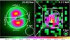 |
Fig. 2 Comparison between the map of the [O iii] surface brightness (left panel, courtesy of Guilin Liu) and the PSF deconvolved, unsmoothed, 0.2–1.0 keV image (right panel). For comparison, a circle with the radius of the core of the Chandra PSF is shown in both panels. In the left panel we show the region that we used to test the symmetry of the soft X-ray extended emission (see the text for details). The color bar of the [O iii] surface-brightness map is also shown. In the right panel we overlay the [O iii] contours on the soft X-ray image. The box represents the area covered by the GEMINI field of view. |
We show all the surface-brightness profiles in Fig. 3. The mismatch between the profile of source (histogram, filled squares) and that of the simulated PSF (dashed line, filled circles) in the first annulus is due to the nuclear pile-up, which artificially lowers the number of counts at low energies. Indeed, the peak of the surface-brightness profile of 1H 0149-577 is consistent with that of PKS 2126-528 (solid line, filled diamonds) which has a similar pile-up fraction. Thus, in our comparisons, the profile of PKS 2126-528 conveniently illustrates how a pile-up of the order of 10% modifies the PSF in the first 2′′. At larger radii, the pile-up has no effects (see e.g., NGC 4151, Wang et al. 2011). The small discrepancy between the profiles of PKS 2126-5128 and those of the simulated PSF could be due to changes of the Chandra-PSF since the time the source was observed (i.e., 1999). Indeed, the build-up of material on the optical blocking filter is known to affect the PSF.
The profile of Fig. 3, left panel, indicates that at energies above 1 keV the source is consistent with being point-like. On the other hand, at energies below 1 keV (right panel), the surface-brightness profile of 1H 0419-577 differs significantly from what is expected from an unresolved point-like source. The profile indicates that, at these energies, the extended emission of the source is resolved by Chandra. The soft X-ray emission of 1H 019-577 appears to be extended up to a distance of 15′′/30 kpc from the center. As we showed in Fig. 1, the bulk of the extended emission comes from a spheroid which extends up to a distance of 8′′/16 kpc. However, beyond this distance, hints of faint filamentary features are seen. These are likely dominating in the tail of the surface-brightness profile.
4. Spectral analysis
 |
Fig. 3 Comparison among the surface-brightness profiles of 1H 0419-577 (histogram, filled squares), those of PKS 2126-158 (solid line, filled diamonds), and those of the Chandra PSF (dashed line, filled circles). We show the comparison in the 1.0–7.0 keV (left panel) and in the 0.2–1.0 keV (right panel) energy bands. All the profiles are background subtracted and normalized to one. We note the logarithmic scale on the vertical axes. |
4.1. The spectrum of the nucleus
In the context of this work, a reliable modeling of the nuclear spectrum is mainly needed to quantify how much the nuclear light scattered by the PSF wings contaminates the spectrum of the extended emission at radii above 2′′. For this purpose, we assume the variably absorbed Comptonization model of Di Gesu et al. (2014). Here, we fitted the spectrum of the nucleus in the 0.7–5.0 keV band. We used two Comptonized components (COMT model in SPEX Titarchuk 1994) where we kept the plasma parameters (temperature T and optical depth τ) frozen to the average of the values observed in the XMM-Newton dataset. Hence, we let the normalizations free to vary. This fit is already statistically acceptable with C/Expected-C = 141/148. However, we checked whether the addition of a neutral absorber could improve the fit. Indeed, the trend between absorbing column density and observed flux that we noticed for the XMM-Newton dataset would predict a column-density of the order of a few 1022 cm-2 at the flux level of the Chandra observation (~8.4 × 10⁻¹² erg s-1 cm-2), which is a low flux state for this source. By adding to the fit a neutral absorber with free column density and covering fraction, we obtained a marginally significant improvement of the fit (ΔC = −8). However, since the obtained parameters of the absorber are in line with the expectation for this flux level, we adopted this case as our best fit for the nuclear spectrum. We show the best-fit model for the spectrum of the nucleus in Fig. 4 and we outline the final best-fit parameters in Table 3.
4.2. Modeling the nuclear contamination at r > 2′′
The spectrum of the nucleus is scattered by the wings of the instrumental PSF at radii larger than the PSF core. As a consequence, any spectrum taken off-nucleus will be slightly contaminated by this scattered light. Here we show, in a model-independent way, that the nuclear spectrum scattered by the PSF wings is not sufficient to explain the spectrum of the extended emission of 1H 0419-577.
In Fig. 5 we plot the ratio between the spectrum taken in the PSF-wing region (between 2′′ and 8′′) and in the PSF-core region (between 0′′ and 2′′) for 1H 0419-577 and for the point-like source PKS 2126-528. We use the 0.3–2.0 keV band to perform this comparison. For a point-like source such as PKS 2126-528 (histogram), this ratio is roughly a constant because it is, at any energy, simply equal to the instrumental ratio between the PSF wings and the PSF core (i.e., wings_to_core ~ 0.04, see Fig. 5). Conversely, for 1H 0419-577, the ratio steepens up at energy below ~1.0 keV, significantly exceeding what is expected from the scattering at larger radii of the spectrum of the central point-like source. This confirms that an extended emission component is present in the spectrum of 1H 0419-577. In all of the following analyses, we modeled the contribution of the scattered nuclear light in the spectrum of the extended emission using the model of the nuclear spectrum of Sect. 4.1, with the normalizations rescaled by the factor wings_to_core.
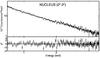 |
Fig. 4 Best-fit for the spectrum of the nucleus (top panel) and spectral residuals in terms of χ2 (bottom panel). The spectrum is shown in the 0.7–5.0 keV band. The solid line represents our best-fit Comptonization model. |
Best-fit parameters for the spectrum of the nucleus. Values without errors were kept frozen in the fit.
4.3. The spectrum of the extended emission
We fitted the spectrum of the extended emission in the 0.3–7.0 keV band. A model including only the rescaled nuclear spectrum adequately fits the data only at energies above 1 keV (Fig. 6), where indeed the source is unresolved (Sect. 3.2). The C-statistics for this model over the 0.3–7.0 keV band is poor (C/Expected-C = 430/45), which confirms a need for some additional extended component at low-energies.
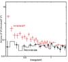 |
Fig. 5 Ratios between the spectrum taken between 0′′ and 2′′ and between 2′′ and 8′′ from the center, for 1H 0419-577 and the point-like source PKS 2126-528. |
At first, we tested whether the spectrum could be due to the thermal emission from a hot, collisionally ionized plasma. For this, we used the CIE model in SPEX which is based on the plasma calculations of Kaastra et al. (1996). The free parameters of the model are the electron temperature (Te) and the emission measure of the plasma Norm. We consider an isothermal plasma with zero turbulent velocity. The default metal abundances in SPEX are protosolar abundances from Lodders et al. (2009).
The addition of a CIE component with Te ~ 0.22 keV (hereafter warm CIE) resulted in a statistically significant improvement of the goodness of the fit. However, the C-statistic for this model (C/Expected-C = 191/45) remains poor. Indeed, the spectrum rises up sharply towards lower energies, significantly exceeding what is expected from a single-temperature plasma (Fig. 6, left panel). Thus, we added another CIE component (hereafter cold CIE) to the fit. We found that the spectrum in the 0.3–7.0 keV band is best-fitted (C/Expected-C = 56/45) by the combination of a warm and cold (Te ~ 0.02 keV) CIE component, besides the contribution of the nuclear spectrum scattered by the PSF wings. The decrease of the C-statistic due to the addition of the cold CIE component is ΔC = −135. In Table 4, upper panel, we list all the parameters and the errors for this model.
Photoionization by the central AGN is another possible physical scenario for the extended emission in Seyfert galaxies. The latest version of SPEX includes for the first time a model for a photoionized plasma in emission. In this PION2 model (Mehdipour et al. 2016), the photoionization equilibrium of the plasma is computed self-consistently using the same continuum of the fit as ionizing SED. In our case, we set the rescaled nuclear continuum as the PION ionizing continuum. The free parameters of this model are the hydrogen column density of the plasmaNHand the ionization parameter log ξ. We noted that, in our fits,NHis degenerate with the Ω parameter in PION, that is a scaling factor related to the geometry of the emitting plasma. Thus, for practical reasons, we considered a spherical shell of material covering the entire sky and a low optical depth plasma out of which both forward and backward radiations can escape (Ω = 2, mix = 0.5). We considered only the emission from the plasma, thus we set a null covering fraction in absorption.
At first we tested if line-emission from a plasma with the same parameters (log NH = 19.9 cm-2, log ξ = 0.03 erg cm s-1) of the known WA could account for the observed extended emission. We found that, in the assumed geometry, the emission from the WA is too weak to account for extended emission. The spectrum is poorly fitted (C = 438/66) and large residuals are left below 1 keV. From this exercise, we conclude that the counterpart in emission of the WA can account at most for 2% of the 0.5–2.0 keV luminosity of the extended emission.
Thus, after having established that plasma parameters different from those of the WA are needed, we letNHand log ξ free to vary in the fit. The behavior of this photoionized plasma model (Fig. 6, right panel) is similar to what we described above for the case of a collisionally ionized plasma model. A single PION component with log ξ = 1.29 (hereafter warm PION) is unable to model the steepening-up of the spectrum at low-energies (C/Expected-C = 206/43). We obtained the best fit (C/Expected-C = 72/43) by adding a second PION component with a lower ionization parameter (log ξ = −4, hereafter cold PION). We outline the parameters and the errors for the final best-fit model in Table 4, lower panel.
In conclusion, this fitting exercise indicates that the extended emission in 1H 0419-577 is consistent with both thermal emission from a hot plasma and with photoionized emission from a warm plasma. Although the C-statistic shows a preference for a collisionally ionized plasma model, a photoionized plasma model cannot be ruled out. In the following, we discuss the physical plausibility of both scenarios, considering the large scale outflow that is known for this AGN.
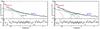 |
Fig. 6 Best-fits of the spectrum of the extended emission using a collisionally ionized plasma model (left panel) and a photoionized plasma model (right panel). In each panel, we show the total best-fit model (solid line), the spectral components separately (dotted lines), and the residuals in terms of χ2. The spectral components are labeled as in Table 4. |
5. Discussion
We present here an analysis of a high-spatial-resolution Chandra ACIS-S image of the bright quasar 1H 0419-577. We find that the source is resolved for energies below ~1 keV. Extended soft X-ray emission is detected up to a distance of at least ~8′′/16 kpc from the nucleus. The 0.5–2.0 keV luminosity in the extended emission is ~2 × 1042 erg s-1. Our finding confirms a previous detection of extended emission with ROSAT-HRI (Predehl & Prieto 2001).
We can certainly exclude that the extended X-ray emission is an artifact due to the scattering of the source X-ray photons by the dust in our Galaxy (Predehl & Schmitt 1995). The foreground dust reddening along the line of sight of 1H 0419-577 (E(B−V) = 0.015) is similar to that of the nearby Seyfert NGC 4051, for example. This corresponds to a lowNHalong our line of sight and thus, no evident X-ray scattering halo is expected. Indeed, in the Chandra ACIS-S image of NGC 4051, no strong extended emission is present (Uttley et al. 2003).
Moreover, we can exclude that we are observing a virialized hot gas halo similar to those which are often seen in early-type galaxies (Forman et al. 1979). For these hot gas halos the soft X-ray luminosity is tightly correlated with the gas temperature (O’Sullivan et al. 2003). For a gas temperature of ~0.2 keV, as we found here for 1H 0419-577, this scaling relationship predicts a luminosity of ~9 × 1039 erg s-1. This is at least two orders of magnitude lower than the luminosity that we find here for the extended emission.
Thus, after having excluded other possibilities, the prime suspect for being related with the extended soft X-ray emission is the galactic-scale [O iii] outflow, that is also seen as a WA in the X-ray/UV spectrum. Galactic winds can be initially driven either by a powerful AGN disk wind (King 2010) or by the combination of stellar winds and supernovae associated to a starburst (Heckman et al. 1990). In the case of 1H 0519-577, the photoionization in the [O iii] outflow is certainly dominated by the AGN, rather than by the SF. Indeed, Liu et al. (2015) find that the ratio between the [O iii] and the Hβ line is constantly above 10, up to a distance of ~5 kpc from the nucleus. This line ratio indicates AGN dominance according to the classification of Baldwin et al. (1981). However, in principle, the SF may still be the driver of the kinetic outflow. Using the relationship given in Rieke et al. (2009) and the Spitzer-MIPS luminosity at 24 μm (~9 × 10¹⁰L⊙, Capak et al. 2012), we estimated a star formation rate of SFR ≲ 70M⊙ yr-1 for 1H 0419-577. We consider the obtained value to be an upper limit because the calculation assumes that the infrared luminosity is only due to the SF, while in reality the nucleus (i.e., the dusty torus surrounding the nucleus) certainly contributes to a fraction of it. The true SFR is likely even lower than this. Indeed, in the near infrared, the source displays an AGN-dominated spectrum, lacking a prominent polycyclic aromatic hydrocarbon (PAH) feature at 3.3 μm (LPAH 3.3 μm ≤ 4.5 × 10⁸L⊙, Yamada et al. 2013). These PAH molecules are considered a good indicator of star formation activity in AGN hosts (e.g., Shi et al. 2007).
According to the computations of Veilleux et al. (2005), for example, a constant SFR, at a time t ~ 107 yr, can produce at most a wind kinetic luminosity of ~7 × 1041 erg s-1for each solar mass of star formed. Thus, in our case this implies Lkin ≲ 5 × 1043 erg s-1, which is in principle consistent with the kinetic luminosity estimated for the [O iii] outflow ([0.01−7] × 1043 erg s-1, Liu et al. 2015). Hence, we cannot exclude that the SF drives or contributes in driving the galactic outflow. We can, however, exclude that the X-ray luminosity of the extended emission is due to the combination of high-mass X-ray binaries, young supernova remnants, and hot plasma associated to the starburst. If that was the case, according to the relationship of Ranalli et al. (2003), the expected soft X-ray luminosity would be L0.5−2.0 keV ≲ 3 × 1041 erg s-1. This is at least one order of magnitude lower that the luminosity that we measured for the extended emission.
Parameters for two for the spectrum of the extended emission.
In our spectral analysis we tested both a collisional-ionization and a photoionization scenario for the physical origin of the extended emission. Both models predict emission lines that could be, in principle, individually resolved in a higher-resolution spectrum. We used the RGS spectrum that we published in Di Gesu et al. (2013) to check if the features predicted by our models of the extended emission are consistent, within the errors, with higher-resolution spectral data. For this exercise we recorded the luminosities predicted by the CIE/PION model for the most prominent X-ray transitions and we compare them with the measured line luminosities or upper limits derived from the RGS data. We list all the predicted and observed line luminosities in Table 5.
Comparison between the predicted and the observed luminosities of the emission lines of the extended emission component.
We found that the cold component PION/CIE model predicts strong emission lines from lowly ionized carbon and nitrogen that are not present in the data (Table 5, upper panel). We note, however, that the ACIS effective area in the energy range where the cold PION/CIE component dominates the spectrum is affected by high uncertainty due to a time-dependent molecular contamination which has been building up on the optical filters. This is most likely preventing us from achieving a reliable parameterization of the model in this energy range. An observation using the Low Energy Transmission Grating Spectrometer in combination with the HRC detector would be best suited to studying the spectrum in the low-energy range. Conversely, we found that all the emission lines predicted by the warm component of the PION/CIE model are consistent with the RGS data (Table 5, lower panel). Thus, after this test, both a collisionally ionized and a photoionized plasma model remain plausible explanations for the spectrum of the extended emission at energies comprised between ~0.5 and ~1.0 keV.
In the case of the collisionally ionized model, the normalization of the CIE model nenHV (where ne and nH are the electron and proton density, respectively, and V is the volume of the emitting gas) provides an estimate of the gas density. Assuming a filled sphere with a radius of 16 kpc, we obtain a gas number density of the order of 10-3 cm-3. Such a low-density hot medium may be a shocked gas component associated to the galactic wind. Analytical models for AGN feedback (Faucher-Giguère & Quataert 2012; King & Pounds 2015) prescribe that a powerful nuclear wind, initially driven by the activity of the central supermassive black hole, collides with the surrounding medium and drives an outflow. Because of the impact, a backwards shock propagates in the wind, while a forward shock is driven into the surrounding ISM. The shocked, expanding ISM is expected to cool radiatively (Zubovas & King 2014; Costa et al. 2015) from temperatures of the order of 107 K down to temperatures of the order of 104 K. As the shock propagates outward, free-free emission becomes the prevailing cooling mechanism and X-ray luminosities comprised between 1041 and 1044 erg s-1, where the exact value depends mainly on the location of the shock radius and on the density of the ambient medium, are predicted (Nims et al. 2015).
This interpretation has also been proposed for the case of SDSS J1356+1026 (Greene et al. 2014) which is another quasar where both a galactic-scale [O iii] outflow and an extended soft X-ray emitting nebula were detected. In this scenario, the [O iii] and the X-ray/UV WA may trace clouds of colder swept-up material that are entrained in the wind. A two-phase wind structure, where the line-emitting gas is confined to colder clumps that are in pressure equilibrium with a hot, low-density outflow, has been proposed for instance in Liu et al. (2013) to explain the observed properties of ~kpc scale [O iii] outflow in radio-quiet quasars. The warm photoionized gas may be in pressure equilibrium with the hot medium if nwarmTwarm ~ nhotThot. Using the parameters derived here for the hot gas and taking Twarm ~ 104 K for the photoionized gas, the pressure equilibrium condition prescribes nwarm ~ 0.1 cm-3. This is in principle compatible with the upper limit for the WA density derived in Edmonds et al. (2011) and with that derived in Liu et al. (2015) for the [O iii]-emitting material.
On the other hand, we cannot rule out the possibility that we are instead observing a nebula of photoionized gas. The AGN is able to photoionize the gas up to a scale of a tenth of a parsec, thus a photoionized gas nebula extending up to ~16 kpc is conceivable. In this scenario, a morphological correspondence between the [O iii] and the soft X-ray emission is expected. In our case, a higher resolution in the soft X-ray band would be needed to access the true morphology at scales comparable to the size of [O iii] lobes. Nevertheless, we attempted to perform a comparison using a PSF deconvolved image (as in e.g., Gómez-Guijarro et al. 2017) and, in this exercise, we found that the soft X-ray and the [O iii] morphology do not match. If confirmed, this lack of morphological correspondence could indicate that the [O iii] line and the soft X-ray emission do no not arise in the same photoionized medium.
In addition, we found that the counterpart in emission of the WA can account only for a small fraction (~2%) of the extended emission luminosity. Thus, the present analysis confirms that a connection between the line-emitting gas and X-ray/UV WA is unlikely in this case (Di Gesu et al. 2013). Indeed, the global parameters of the emitting (i.e., log NH ~ 22.3 cm-2 and log ξ ~ 1.3 erg cm s-1) and of the absorbing (i.e., log NH ~ 19.9 cm-2 and log ξ ~ 0.03 erg cm s-1) gas are largely inconsistent. This implies that the extended photoionized emitting gas must have a low covering fraction for absorption. Indeed, a photoionized gas with the parameters found here is expected to produce prominent absorption lines (e.g., O vii-O viii, Fe-UTA) in the RGS band, that are not present in the data In Di Gesu et al. (2013) we performed the photoionization modeling of the UV/X-ray narrow emission lines in this source. In that exercise, we found a covering fraction of 4% for the emitting gas. If we use this value of covering factor for the PION component found here, the associated absorption lines are indeed consistent with the Chandra-ACIS and the RGS data. Such a low-covering fraction implies that either the gas is fragmented in small clouds or that it is mostly outside our line of sight. Liu et al. (2015) found that the rotational pattern suggested by the median velocity of the [O iii] line is suggestive of disk galaxy viewed almost edge-on (≥70°). Moreover, in Di Gesu et al. (2014) we proposed that the AGN is seen at high inclination. In this geometry, in order not to intercept our line of sight, the photoionized soft X-ray emitting gas must be distributed mostly along the polar directions, rather than being spherically symmetrical. If this was the case the UV/X-ray WA, must trace a different gas component, physically disconnected from the emitting gas, and located closer to the equatorial plane.
6. Summary and conclusion
We analyzed a Chandra-ACIS high-spatial-resolution image of the Seyfert 1 galaxy 1H 0419-577. This source is known for hosting a galactic-scale outflow, which is seen as warm absorber in the UV and in the X-ray spectrum, and is also highlighted in the [O iii] image.
Extranuclear X-ray emission is resolved by Chandra at energies lower than 1 keV. The bulk of the soft X-ray emission comes from a roughly spherically symmetrical halo surrounding the nucleus. This extends up to a distance of ~8′′/16 kpc and has a luminosity of ~2 × 1042 erg s-1in the 0.5–2.0 keV band.
The morphology of the soft X-ray extended emission is spherically symmetric. We were unable to recover a morphological resemblance between the soft X-ray extended emission and the biconical outflow that is traced by the [O iii] emission line.
The analysis of the spectrum of the extended emission did not yield conclusive results about its physical origin. We report that the spectrum rises up sharply at energies below ~0.5 keV. However, due to the calibration uncertainty of the ACIS effective area in this energy range, we are unable to find an accurate parameterization of any model in this spectral range.
In the energy range between 0.5 end 1 keV, both a collisionally ionized (Te = 0.22 ± 0.02 keV) and a photoionized plasma-model (log ξ = 1.3 ± 0.1, NH = 2.1 ± 0.5 × 1022 cm-2) best-fit the ACIS spectrum and are consistent with the RGS spectrum already published in Di Gesu et al. (2013).
In the former case, we may be observing a thermally emitting gas bubble, which was inflated by the wind shock and that is radiatively cooling down. In this scenario the [O iii] emission line and the X-ray/UV warm absorber may trace cooler clumps that are entrained in the hot wind.
Alternatively, we may be observing a large-scale photoionized gas nebula. In this case, we can exclude that the extended photoionized gas is the counterpart in emission of the X-ray/UV warm absorber. Thus, we infer that the extended photoionized gas nebula must have a low covering fraction for absorption. This implies that either the gas is fragmented or that it is distributed mostly along the polar directions, outside our line of sight.
See the ROSAT calibration document in the MPA website (http://www.mpe.mpg.de/xray/wave/rosat/calibration/hri/psf/hri_psf.php).
See the SPEX manual: http://var.sron.nl/SPEX-doc/manualv3.02/manual.html
Acknowledgments
The scientific results reported in this article are based on observations made by the Chandra X-ray Observatory. L.D.G. acknowledges support from the Swiss National Science Foundation. SRON is financially supported by NWO, The Netherlands organization for Scientific Research. We thank Guilin Liu for kindly providing the GEMINI-IFU image, and Francesco Tombesi for useful discussions.
References
- Baldwin, J. A., Phillips, M. M., & Terlevich, R. 1981, PASP, 93, 5 [NASA ADS] [CrossRef] [EDP Sciences] [Google Scholar]
- Behar, E., Peretz, U., Kriss, G. A., et al. 2017, A&A, 601, A17 [NASA ADS] [CrossRef] [EDP Sciences] [Google Scholar]
- Bianchi, S., Guainazzi, M., & Chiaberge, M. 2006, A&A, 448, 499 [NASA ADS] [CrossRef] [EDP Sciences] [Google Scholar]
- Capak, P. L., Teplitz, H., Hanish, D., et al. 2012, in American Astronomical Society Meeting Abstracts, 219, 410.01 [Google Scholar]
- Cash, W. 1979, ApJ, 228, 939 [NASA ADS] [CrossRef] [Google Scholar]
- Costa, T., Sijacki, D., & Haehnelt, M. G. 2015, MNRAS, 448, L30 [NASA ADS] [CrossRef] [Google Scholar]
- Crenshaw, D. M., & Kraemer, S. B. 2012, ApJ, 753, 75 [NASA ADS] [CrossRef] [Google Scholar]
- Crenshaw, D. M., Kraemer, S. B., & George, I. M. 2003, ARA&A, 41, 117 [NASA ADS] [CrossRef] [Google Scholar]
- Detmers, R. G., Kaastra, J. S., & McHardy, I. M. 2009, A&A, 504, 409 [NASA ADS] [CrossRef] [EDP Sciences] [Google Scholar]
- Di Gesu, L., Costantini, E., Arav, N., et al. 2013, A&A, 556, A94 (Paper I) [NASA ADS] [CrossRef] [EDP Sciences] [Google Scholar]
- Di Gesu, L., Costantini, E., Piconcelli, E., et al. 2014, A&A, 563, A95 [NASA ADS] [CrossRef] [EDP Sciences] [Google Scholar]
- Di Matteo, T., Springel, V., & Hernquist, L. 2005, Nature, 433, 604 [NASA ADS] [CrossRef] [PubMed] [Google Scholar]
- Ebrero, J., Kaastra, J. S., Kriss, G. A., et al. 2016, A&A, 587, A129 [NASA ADS] [CrossRef] [EDP Sciences] [Google Scholar]
- Edmonds, D., Borguet, B., Arav, N., et al. 2011, ApJ, 739, 7 [NASA ADS] [CrossRef] [Google Scholar]
- Faucher-Giguère, C.-A., & Quataert, E. 2012, MNRAS, 425, 605 [NASA ADS] [CrossRef] [Google Scholar]
- Feruglio, C., Fiore, F., Carniani, S., et al. 2015, A&A, 583, A99 [NASA ADS] [CrossRef] [EDP Sciences] [Google Scholar]
- Fischer, T. C., Crenshaw, D. M., Kraemer, S. B., & Schmitt, H. R. 2013, ApJS, 209, 1 [NASA ADS] [CrossRef] [Google Scholar]
- Forman, W., Schwarz, J., Jones, C., Liller, W., & Fabian, A. C. 1979, ApJ, 234, L27 [NASA ADS] [CrossRef] [Google Scholar]
- Gómez-Guijarro, C., González-Martín, O., Ramos Almeida, C., Rodríguez-Espinosa, J. M., & Gallego, J. 2017, MNRAS, 469, 2720 [NASA ADS] [CrossRef] [Google Scholar]
- Gonzalez-Martin, O., Acosta-Pulido, J. A., Perez Garcia, A. M., & Ramos Almeida, C. 2010, ApJ, 723, 1748 [NASA ADS] [CrossRef] [Google Scholar]
- Greene, J. E., Pooley, D., Zakamska, N. L., Comerford, J. M., & Sun, A.-L. 2014, ApJ, 788, 54 [NASA ADS] [CrossRef] [Google Scholar]
- Guainazzi, M., & Bianchi, S. 2007, in The Central Engine of Active Galactic Nuclei, eds. L. C. Ho, & J.-W. Wang, ASP Conf. Ser., 373, 467 [Google Scholar]
- Guainazzi, M., Comastri, A., Stirpe, G. M., et al. 1998, A&A, 339, 327 [NASA ADS] [Google Scholar]
- Heckman, T. M., Armus, L., & Miley, G. K. 1990, ApJS, 74, 833 [NASA ADS] [CrossRef] [Google Scholar]
- Hopkins, P. F., & Elvis, M. 2010, MNRAS, 401, 7 [NASA ADS] [CrossRef] [Google Scholar]
- Iwasawa, K., Wilson, A. S., Fabian, A. C., & Young, A. J. 2003, MNRAS, 345, 369 [NASA ADS] [CrossRef] [Google Scholar]
- Kaastra, J. S. 2017, A&A, 605, A51 [NASA ADS] [CrossRef] [EDP Sciences] [Google Scholar]
- Kaastra, J. S., Mewe, R., & Nieuwenhuijzen, H. 1996, in UV and X-ray Spectroscopy of Astrophysical and Laboratory Plasmas, eds. K. Yamashita, & T. Watanabe, 411 [Google Scholar]
- Kalberla, P. M. W., Burton, W. B., Hartmann, D., et al. 2005, A&A, 440, 775 [NASA ADS] [CrossRef] [EDP Sciences] [Google Scholar]
- King, A. R. 2010, MNRAS, 402, 1516 [NASA ADS] [CrossRef] [Google Scholar]
- King, A., & Pounds, K. 2015, ARA&A, 53, 115 [Google Scholar]
- Liu, G., Zakamska, N. L., Greene, J. E., Nesvadba, N. P. H., & Liu, X. 2013, MNRAS, 430, 2327 [NASA ADS] [CrossRef] [Google Scholar]
- Liu, G., Arav, N., & Rupke, D. S. N. 2015, ApJS, 221, 9 [NASA ADS] [CrossRef] [Google Scholar]
- Lodders, K., Palme, H., & Gail, H.-P. 2009, in Landolt-Börnstein – Group VI Astronomy and Astrophysics Numerical Data and Functional Relationships in Science and Technology Volume, ed. J. E. Trümper, 44 [Google Scholar]
- Lucy, L. B. 1974, AJ, 79, 745 [NASA ADS] [CrossRef] [Google Scholar]
- McKernan, B., Yaqoob, T., & Reynolds, C. S. 2007, MNRAS, 379, 1359 [NASA ADS] [CrossRef] [Google Scholar]
- Mehdipour, M., Kaastra, J. S., & Kallman, T. 2016, A&A, 596, A65 [NASA ADS] [CrossRef] [EDP Sciences] [Google Scholar]
- Nims, J., Quataert, E., & Faucher-Giguère, C.-A. 2015, MNRAS, 447, 3612 [NASA ADS] [CrossRef] [Google Scholar]
- Nucita, A. A., Guainazzi, M., Longinotti, A. L., et al. 2010, A&A, 515, A47 [NASA ADS] [CrossRef] [EDP Sciences] [Google Scholar]
- O’Sullivan, E., Ponman, T. J., & Collins, R. S. 2003, MNRAS, 340, 1375 [NASA ADS] [CrossRef] [Google Scholar]
- Page, K. L., Pounds, K. A., Reeves, J. N., & O’Brien, P. T. 2002, MNRAS, 330, L1 [NASA ADS] [CrossRef] [Google Scholar]
- Pal, M., & Dewangan, G. C. 2013, MNRAS, 435, 1287 [NASA ADS] [CrossRef] [Google Scholar]
- Piconcelli, E., Jimenez-Bailón, E., Guainazzi, M., et al. 2005, A&A, 432, 15 [NASA ADS] [CrossRef] [EDP Sciences] [Google Scholar]
- Pogge, R. W. 1988, ApJ, 332, 702 [NASA ADS] [CrossRef] [Google Scholar]
- Pounds, K. A., Reeves, J. N., Page, K. L., & O’Brien, P. T. 2004a, ApJ, 605, 670 [NASA ADS] [CrossRef] [Google Scholar]
- Pounds, K. A., Reeves, J. N., Page, K. L., & O’Brien, P. T. 2004b, ApJ, 616, 696 [NASA ADS] [CrossRef] [Google Scholar]
- Predehl, P., & Prieto, A. 2001, ArXiv e-prints [arXiv:astro-ph/0109542] [Google Scholar]
- Predehl, P., & Schmitt, J. H. M. M. 1995, A&A, 293, 889 [NASA ADS] [Google Scholar]
- Ranalli, P., Comastri, A., & Setti, G. 2003, A&A, 399, 39 [NASA ADS] [CrossRef] [EDP Sciences] [Google Scholar]
- Rieke, G. H., Alonso-Herrero, A., Weiner, B. J., et al. 2009, ApJ, 692, 556 [NASA ADS] [CrossRef] [Google Scholar]
- Rupke, D. S. N., & Veilleux, S. 2013, ApJ, 768, 75 [NASA ADS] [CrossRef] [Google Scholar]
- Shi, Y., Ogle, P., Rieke, G. H., et al. 2007, ApJ, 669, 841 [NASA ADS] [CrossRef] [Google Scholar]
- Singh, K. P., Garmire, G. P., & Nousek, J. 1985, ApJ, 297, 633 [NASA ADS] [CrossRef] [Google Scholar]
- Smith, D. A., & Wilson, A. S. 2001, ApJ, 557, 180 [NASA ADS] [CrossRef] [Google Scholar]
- Titarchuk, L. 1994, ApJ, 434, 570 [NASA ADS] [CrossRef] [Google Scholar]
- Turner, T. J., Miller, L., Kraemer, S. B., Reeves, J. N., & Pounds, K. A. 2009, ApJ, 698, 99 [NASA ADS] [CrossRef] [Google Scholar]
- Uttley, P., Fruscione, A., McHardy, I., & Lamer, G. 2003, ApJ, 595, 656 [NASA ADS] [CrossRef] [Google Scholar]
- Veilleux, S., Cecil, G., & Bland-Hawthorn, J. 2005, ARA&A, 43, 769 [Google Scholar]
- Veilleux, S., Teng, S. H., Rupke, D. S. N., Maiolino, R., & Sturm, E. 2014, ApJ, 790, 116 [NASA ADS] [CrossRef] [Google Scholar]
- Véron-Cetty, M.-P., & Véron, P. 2006, A&A, 455, 773 [NASA ADS] [CrossRef] [EDP Sciences] [Google Scholar]
- Wang, J., Fabbiano, G., Elvis, M., et al. 2009, ApJ, 694, 718 [NASA ADS] [CrossRef] [Google Scholar]
- Wang, J., Fabbiano, G., Risaliti, G., et al. 2010, ApJ, 719, L208 [NASA ADS] [CrossRef] [Google Scholar]
- Wang, J., Fabbiano, G., Risaliti, G., et al. 2011, ApJ, 729, 75 [NASA ADS] [CrossRef] [Google Scholar]
- Wang, J., Nardini, E., Fabbiano, G., et al. 2014, ApJ, 781, 55 [NASA ADS] [CrossRef] [Google Scholar]
- Whewell, M., Branduardi-Raymont, G., Kaastra, J. S., et al. 2015, A&A, 581, A79 [NASA ADS] [CrossRef] [EDP Sciences] [Google Scholar]
- Whewell, M., Branduardi-Raymont, G., & Page, M. J. 2016, A&A, 595, A85 [NASA ADS] [CrossRef] [EDP Sciences] [Google Scholar]
- Yamada, R., Oyabu, S., Kaneda, H., et al. 2013, PASJ, 65, 103 [NASA ADS] [Google Scholar]
- Young, A. J., Wilson, A. S., & Shopbell, P. L. 2001, ApJ, 556, 6 [NASA ADS] [CrossRef] [Google Scholar]
- Zubovas, K., & King, A. R. 2014, MNRAS, 439, 400 [NASA ADS] [CrossRef] [Google Scholar]
All Tables
Comparison between the soft X-ray surface brightness inside and outside the [O iii] outflow regions.
Best-fit parameters for the spectrum of the nucleus. Values without errors were kept frozen in the fit.
Comparison between the predicted and the observed luminosities of the emission lines of the extended emission component.
All Figures
|
Fig. 1 Chandra-ACIS images of 1H 0419-577 (top left) and of the point-like source PKS 2126-158 (top right) in the 0.2–1.0 keV band. As a visual aid, we also show the color bar of these two images at the bottom. For comparison, we show in both the panels a circle with the radius of the core of the Chandra PSF. Bottom left: same as first panel, smoothed using a Gaussian kernel of 3 pixels. The regions that we used for spectral extraction are overlaid. We also mark the direction from which we removed the ACIS readout streak (dashed line) and the location of possible extended filaments around the source. Bottom right: false-color image obtained using the PSF-deconvolved 0.2–0.5, 0.5–2.0, and 2.0–7.0 keV band images as red, green, and blue, respectively. |
| In the text | |
|
Fig. 2 Comparison between the map of the [O iii] surface brightness (left panel, courtesy of Guilin Liu) and the PSF deconvolved, unsmoothed, 0.2–1.0 keV image (right panel). For comparison, a circle with the radius of the core of the Chandra PSF is shown in both panels. In the left panel we show the region that we used to test the symmetry of the soft X-ray extended emission (see the text for details). The color bar of the [O iii] surface-brightness map is also shown. In the right panel we overlay the [O iii] contours on the soft X-ray image. The box represents the area covered by the GEMINI field of view. |
| In the text | |
|
Fig. 3 Comparison among the surface-brightness profiles of 1H 0419-577 (histogram, filled squares), those of PKS 2126-158 (solid line, filled diamonds), and those of the Chandra PSF (dashed line, filled circles). We show the comparison in the 1.0–7.0 keV (left panel) and in the 0.2–1.0 keV (right panel) energy bands. All the profiles are background subtracted and normalized to one. We note the logarithmic scale on the vertical axes. |
| In the text | |
|
Fig. 4 Best-fit for the spectrum of the nucleus (top panel) and spectral residuals in terms of χ2 (bottom panel). The spectrum is shown in the 0.7–5.0 keV band. The solid line represents our best-fit Comptonization model. |
| In the text | |
|
Fig. 5 Ratios between the spectrum taken between 0′′ and 2′′ and between 2′′ and 8′′ from the center, for 1H 0419-577 and the point-like source PKS 2126-528. |
| In the text | |
|
Fig. 6 Best-fits of the spectrum of the extended emission using a collisionally ionized plasma model (left panel) and a photoionized plasma model (right panel). In each panel, we show the total best-fit model (solid line), the spectral components separately (dotted lines), and the residuals in terms of χ2. The spectral components are labeled as in Table 4. |
| In the text | |
Current usage metrics show cumulative count of Article Views (full-text article views including HTML views, PDF and ePub downloads, according to the available data) and Abstracts Views on Vision4Press platform.
Data correspond to usage on the plateform after 2015. The current usage metrics is available 48-96 hours after online publication and is updated daily on week days.
Initial download of the metrics may take a while.