| Issue |
A&A
Volume 601, May 2017
|
|
|---|---|---|
| Article Number | A121 | |
| Number of page(s) | 9 | |
| Section | Stellar structure and evolution | |
| DOI | https://doi.org/10.1051/0004-6361/201630360 | |
| Published online | 17 May 2017 | |
Does the Wolf-Rayet binary CQ Cephei undergo sporadic mass transfer events?
1 Instituto de Ciencias Físicas, Universidad Nacional Autónoma de México, Ave. Universidad S/N, Cuernavaca, 62210 Morelos, México
e-mail:
This email address is being protected from spambots. You need JavaScript enabled to view it.
2 Physikalisch-Meteorologisches Observatorium Davos and World Radiation Center (PMOD/WRC), Dorfstrasse 33, 7260 Davos Dorf, Switzerland
e-mail:
This email address is being protected from spambots. You need JavaScript enabled to view it.
3 CASA, University of Colorado, Boulder, CO 80309-0389, USA
e-mail:
This email address is being protected from spambots. You need JavaScript enabled to view it.
Received: 26 December 2016
Accepted: 18 February 2017
Abstract
Context. Stellar wind mass-loss in binary systems carries away angular momentum causing a monotonic increase in the orbital period, Ṗ> 0. Despite possessing a significant stellar wind, the eclipsing Wolf-Rayet (WR) binary system CQ Cep does not show the expected monotonic period increase, in fact, it is sometimes reported to display the opposite behavior.
Aims. The objective of this paper is to perform a new analysis of the rate of period change Ṗ and determine the conditions under which Roche-lobe overflow (RLO) mass-transfer combined with wind mass loss can explain the discrepant behavior.
Methods. The historic records of times of light curve minima were reviewed and compared with the theoretical values of Ṗ for cases in which both wind mass-loss and RLO occur simultaneously.
Results. The observational data indicate that Ṗ alternates between positive and negative values on a timescale of years. The negative values (Ṗ ~ −0.6 to −8.5 s yr-1) are significantly larger in absolute value than the positive ones (Ṗ ~ + 0.2 to +1.2 s yr-1). We find that a plausible scenario for CQ Cep is one in which the O star undergoes intense but sporadic RLO events that lead to accretion onto the WR star, at which times Ṗ< 0. At other times, Ṗ> 0 when the WR wind, and possibly material swept up from the O star, carries angular momentum away from the system. A scenario in which the WR star is the mass donor cannot be excluded, but requires that either the WR wind mass-loss rate undergoes large sporadic enhancements or that an additional process that removes angular momentum from the system be present.
Key words: accretion, accretion disks / binaries: eclipsing / stars: individual: CQ Cep / stars: mass-loss / stars: winds, outflows / stars: Wolf-Rayet
© ESO, 2017
1. Introduction
Wolf-Rayet (WR) stars are descendents of massive O-type stars and represent one of the last phases in the evolution of such stars before they explode as supernovae. They are over-luminous for their mass, compared to main sequence stars, and they display chemical abundances indicating substantial enrichment by nuclear-process material in the surface layers. Although they have very intense winds, their current masses are too low to be explained by steady wind mass-loss alone. Hence, massive stars are thought to reach a transition state in which they shed their outer layers through one or a sequence of rapid and intense mass-ejection events before reaching the WR state (Puls et al. 2008). There are two identified modes by which such mass-loss may occur. The first takes place while the star is still on the blue side of the Hertzprung-Russel Diagram and is associated with the type of outbursts that are observed in the luminous blue variable (LBV) stars. However, the mechanism causing the outbursts has not been established, nor is it known to occur primarily in binary systems. The second mode involves mass transfer or loss via Roche-lobe overflow (RLO) in a binary system (see Langer 2012, and references therein). In short-period systems, the more massive component is the first to undergo RLO, followed some time later by a similar event in its (originally) lower mass companion (Vanbeveren et al. 1997).
The computed evolutionary path of a binary star is strongly dependent on the amount of matter and angular momentum that is exchanged or lost, and on the evolutionary phase at which this event occurs (Paczyński 1971; Podsiadlowski et al. 1992; De Loore & Vanbeveren 1994; Nelson & Eggleton 2001; Hurley et al. 2002; Wellstein et al. 2001; Shao & Li 2016). Many currently observed binary systems are believed to be the product of RLO during the recent past, for example, Algols and chemically-peculiar O+O systems such as HD 149404 (Raucq et al. 2016), among many others. However, only a limited number of non-compact companion systems have been observed at a time in which unambiguous indications of RLO are observed. Examples include HR 5171 A (Chesneau et al. 2014) and RY Scuti (Smith et al. 2011; Antokhina & Cherepashchuk 1988).
CQ Cep (=WR 155 = HD 214419) is a galactic WR star of the subtype WN6 in a close orbit with a O9II-Ib star (Marchenko et al. 1995). Its orbital period P = 1.64d is one of the shortest known among WR binaries.
The WN6-type spectrum consists of broad high-ionization emission lines which are a clear diagnostic for wind mass-loss. The mass-loss rates were derived independently by Cherepashchuk (1982), Howarth & Schmutz (1992) and Nishimaki et al. (2008) and are consistent with a value 2 ± 1 × 10⁻⁵M⊙ yr-1. An additional determination by Hamann & Koesterke (1998) yielded a somewhat larger value, 5 × 10⁻⁵M⊙ yr-1. We give in Table 1 a summary of CQ Cep’s parameters as derived by Demircan et al. (1997), Marchenko et al. (1995) and Harries & Hilditch (1997), referred to hereafter as D97, M95, HH97 respectively.
The wind mass-loss is expected to produce an increase over time of the orbital period in the range Ṗ ~ 0.07–0.2 s yr-1 (Khaliullin 1974). However, the analyses of CQ Cep’s light curves by Gaposchkin (1944) and Semeniuk (1968) result in the contrary conclusion, as do Antokhina et al. (1982; Ṗ = −0.019 ± 0.006 s yr-1) and Cherepashchuk (1982; Ṗ = −0.038 s yr-1). The latter authors conclude that the dominant process in CQ Cep is one in which mass is being transferred from the WR star to the companion (assuming that the WR star is the more massive of the two stars in the system). However, Kreiner & Tremko (1983) conclude that although the orbital period may have been variable prior to 1942, it remained relatively constant thereafter, which could be explained if the angular momentum loss due to wind mass-loss and the increase due to mass transfer between the two components balanced each other. Walker et al. (1983) arrived at a similar conclusion. An alternative scenario put forth by Kurochkin in 1979 as cited by Antokhina et al. (1982) and Kreiner & Tremko (1983) is that the rate of period change alternates between positive and negative values, which could be explained if mass-transfer due to RLO occurred only sporadically.
Given the above, CQ Cep presents an outstanding opportunity for studying the interplay between stellar wind mass-loss and mass-transfer in a high mass binary system, if indeed this is the phenomenon that is causing the peculiar behavior in Ṗ. Thus, the objective of this paper is to determine the conditions under which such an interplay may be present in CQ Cep.
In Sect. 2 we present a critical review of the historic records of times of the light curve minima observed over approximately seven decades in order to establish whether or not period changes are present. In Sect. 3 we analyze the conditions that may lead to an alternating sign in Ṗ. The discussion and conclusions are, respectively, in Sects. 4 and 5.
CQ Cep parameters.
2. The variations in 
The light curve of CQ Cep presents two clear eclipses, and thanks to its very short orbital period and relative brightness, photographic and photoelectric light curves have been published since the early 1940s. The time elapsed between successive primary light curve minima has thus allowed a precise determination of the orbital period and, at the same time, an assessment of the differences between the time at which an observed minimum is expected and the time it is actually observed; that is, the quantity O−C. As mentioned above, contradictory results for the trend of O−C over time have been derived. Walker et al. (1983) presented a comprehensive analysis of the light curve shape and discussed the manner in which its variations over time introduce a larger than usual uncertainty in the measured times of minima. However, even taking into account these larger uncertainties, the increasing trend of O−C over time expected due to wind mass-loss did not emerge.
We revisited the data that are available on the times of minimum in the CQ Cep light curve, making a careful selection of these data on the basis of their reported accuracy. We then calculated the observed minus computed (O−C) times of minima using a fixed reference orbital period. We used the compilation of observation epochs available at the O−C gateway (Paschke & Brat 2006), and limited the analysis to the sequence of minima starting from a reference epoch in the year 1947. This reference epoch, which corresponds to HJD 2 432 456.671, was converted for consistency with newer data from the UTC date given by Hiltner (1950) to Barycentric Julian date using the website http://astroutils.astronomy.ohio-state.edu/time/utc2bjd.html.
All other epochs used here have been converted to barycentric Julian date (BJD) unless it was indicated in the original publication that the given value was already corrected to heliocentric Julian date (HJD), in which case the HJD value was adopted, as the difference between HJD and BJD is ~4s, which is negligible in our context. The sample was limited to the data in which the reported times of minima have uncertainties no larger than ± 0.005d. This is a conservative estimate and takes into account different approaches to determining the minima and possible variable eclipse shapes. In fact, many references list uncertainties as small as ± 0.002d.
The last reported minimum was observed by Chandra in 2013 and reported in Skinner et al. (2015). The extremely smooth observed optical light curve allowed the time of minimum to be measured to within 20 s. The smoothness of the 2013 light curve is in strong contrast to significant light curve variations in September 1982 reported by Walker et al. (1983). The latter estimated that their determination was accurate to 6 min but that individual minima may have been off by as much as 12 min.
The references for the times of minima for epochs from 1947 to the 1980s are the following: Three observations obtained in 1959, 1965, and 1967 were adapted from Table 1 of Kreiner & Tremko (1983), which refer to publications from Tchugainov (1960), Guseinzade (1967), and Kartasheva (1972), to which we did not have access. We have omitted photographic observations obtained in 1953 because the listed error of the epoch is 0.006d. Two minima epochs in 1971 have been obtained from Meyer (1972) who assigned an error of 0.002d and 0.005d, respectively to these two epochs. These uncertainties are particularly relevant because Meyer’s values give the largest deviations in the O−C diagram. Five entries in 1973 and one for 1974 are from Table 1 of Kreiner & Tremko (1983) referenced as private communication with Chis & Pop (1983), and two entries for 1975 referenced to Kartasheva (1976). The O−C gateway lists an additional Kartasheva entry for 1976 that we have also included. The observations were made with a variety of different filters which however, does not seem to be an issue as Stickland et al. (1984) did not find a dependence of the time of primary minimum with wavelength, based on observations obtained in the UV to the visual wavelength range.
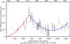 |
Fig. 1 The O−C diagram for the primary minima calculated from the linear elements (Eq. (1)). The abscissa is given in units of orbit number, with the origin defined on HJD 2 432 456.671 (1947 Sept. 28) and adopting P0 = 1.64124d. The ordinate is in units of fraction of orbital period. The error bars indicate an assumed precision of ±0.005 in orbital fraction, which corresponds to ~11 min. The red squares denote values from 1947 to 1971 and the blue diamonds denote data from 1971–2014. The last point corresponds to Skinner et al. (2015), who have determined the time of minimum to a precision of 20 s. |
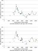 |
Fig. 2 Same as previous figure only that here we illustrate the quadratic fits to portions of the data that display strong variations. Top: fits with positive quadratic coefficients. Bottom: fits with negative quadratic coefficients. (see Table 2 for the corresponding values). Different symbols indicate the O−C values that were used to derive each parabolic fit reported in Table 1. |
The resulting O−C diagram for the primary minima is presented in Fig. 1. The abscissa of the plot gives the integral number of orbital cycles N, starting from the reference initial epoch E0 = HJD 2 432 456.671 (28 September 1947) and using as initial orbital period P0 = 1.64124d. The ordinate was calculated from  (1)where TObs and TC are the times of the observed and the computed minima, respectively. TC was computed with E0 and P0 given above.
The error bars in Fig. 1 indicate an assumed uncertainty of ±0.005 in orbital fraction, which corresponds to ~11 min. From 1947 until the 1960s, the published entries are the average of several minima observations, whereas starting from the 1970s, individual minima observations are given. This appears in the O−C diagram as a larger scatter of the O−C values and a denser coverage in time starting in the 1970s.
A first inspection of Fig. 1 suggested that there is a period lengthening trend during the first 5000 orbits, as well as one over the more recent orbits. As in Walker et al. (1983), we fit these two trends with a least squares fit orthogonal polynomial of the form y = ax2 + bx + c, where x = (T−T0) /P0 and  , with N the number of orbital cycles. Using
  , allows one to write Ṗ/(s/yr)= 2a × 3.1558 × 107. The coefficient of the quadratic term obtained for the data of 1947–1971 is a = 7.0 × 10⁻¹⁰, with a similar value obtained for the 1971–2014 fit. This yields Ṗ ~ + 0.04 s yr-1, which is significantly smaller than predicted for a steady WR wind mass-loss rate ṁ ~ 10-5M⊙ yr-1.
Upon closer inspection of Fig. 1, however, the presence of non-monotonic trends is evident after 1970, which is when the individual times of minima are plotted (as opposed to averages over many times of minima prior to this date). These deviations are even more significant than they appear in Fig. 1 because our adopted maximum uncertainty of 11 min in the value of the minima determinations is very conservative. As mentioned above, we used only data with stated uncertainties ≤0.005d (7 min).
Adopting the hypothesis that non-monotonic variations are present in the (O−C) values, we now fit quadratic functions to the epochs listed in the first column of Table 2. The coefficients of the orthogonal polynomial fits are listed in Cols. 2–4. Column 5 lists the derived value of Ṗ. These are consistent with the presence of transitions from positive to negative values.
Due to the low density of measurements, several of the fits with a positive quadratic term depend critically on only one point and therefore we can only consider these fit curves to provide a rough estimate of the wind mass-loss rate. An exception is the epoch 1971.7–1982.7, for which there are several good quality measured O−C values. The quadratic fit term of this curve yields Ṗ ~ + 0.4 s yr-1. We estimate a 10% uncertainty for this fit.
A similar word of caution as for the fits with positive quadratic terms applies to the fits with negative quadratic terms. For example, the two epochs 1998.4–2006.8 and 2009.8–2013.2 depend on a single O−C value in 2003.6 and 2011.7, respectively. However, the O−C transitions from before and after 1971.7 and before and after 1982.7 undoubtably require a shortening of the period. Furthermore, the magnitude of the negative quadratic terms is likely to give only a lower limit, since the mass transfer events causing Ṗ< 0 might be expected to have a shorter duration than the time interval between observational measurements. In conclusion, we find that the variations in the derived values of Ṗ are consistent with the suggestion of Kurochkin (1979; cited by Antokhina et al. 1982) that Ṗ alternates between positive and negative values.
3. What determines  ?
?
Wind mass-loss, ṁw removes angular momentum from a binary system, leading to a lengthening of the orbital period Ṗ> 0. Mass exchange through RLO can lead to either Ṗ> 0 or Ṗ< 0 depending on the mass ratio of the binary components. Khaliullin (1974) provided a theoretical framework for these different cases. He showed that when the analysis is applied to the WR-system V444 Cyg (WN5+O6; P = 4.2d), the derived value Ṗ = + 0.22 s yr-1 is consistent with a WR star mass-loss rate ṁw = (1.11 ± 0.22) × 10-5M⊙ yr-1, as also obtained from independent spectroscopic diagnostics.
Coefficients of the ax2 + bx + c fits to the O−C diagram and implied Ṗ.
In the case of CQ Cep, however, although there is a clear indication of a stellar wind similar to that of V444 Cyg, the measured times of light curve minima do not support the presence of a similar long-term increase in Ṗ. The natural explanation lies in a combination of wind mass-loss and mass exchange, the latter of which either cancels the angular momentum loss due to ṁw or even exceeds it. In this section we discuss the conditions under which the observed behavior of Ṗ in CQ Cep may be understood within this theoretical framework.
Following Khaliullin (1974), we assume a circular orbit and use, 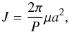 (2)and
 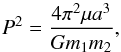 (3)where J is the total orbital angular momentum, P and a are the orbital period and separation, m1, m2 are the masses, G the gravitational constant, and
  the reduced mass. Combining these two equations:
 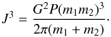 (4)Taking the time derivative of the above and defining q = m1/m2, the following expression for Ṗ/P (Eq. (2) in Khaliullin 1974) is derived:
 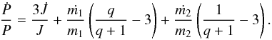 (5)This equation provides the rate of orbital period change over time due to the rate of mass-loss or mass-gain of each of the two stars
  ,
,  , and due to the loss of angular momentum from the system,
  . We note that and can take on either negative or positive values, depending on whether mass is lost or gained by the star. Note also that no assumption is made regarding the stellar masses; that is, q may be either greater or smaller than unity.
We know from the emission-line spectrum in CQ Cep that the WR-star component has a powerful stellar wind and thus, angular momentum is lost from the system. Assuming this is the only source of angular momentum loss and no mass transfer, and assuming a WR wind mass-loss rate  in the range (1−3) × 10-5M⊙ yr-1, Eq. (5) yields Ṗ in the range + 0.05− + 0.16 s yr-1 for the HH97 mass ratio and + 0.07− + 0.20 s yr-1 for the D97 and M95 mass ratio.
If the wind mass-loss remains relatively constant with time, Eq. (5) predicts a monotonic change in P, implying Ṗ = constant. This holds true even if a fraction of the wind is captured by the O star since there is no reason to assume that this fraction varies over time. Thus, in order to produce non-monotonic variations in Ṗ, there must be mass exchange in addition to the wind mass-loss of the WR star. This is a feasible hypothesis because the dimensions of the WR and the O star, derived from the eclipse light curves, are close to their corresponding Roche radii. In fact, if we substitute the nominal masses (Table 1) and radii that have been estimated for each of the two stars in CQ Cep into the analytic approximation for Roche radii RRL given by Eggleton (1983), we find that in all cases the O-star and the WR-star radii exceed RRL1 . Furthermore, it is possible to estimate the shortest period possible that a binary of mass ratio q can have without overflowing the Roche Lobe (Eggleton 2002), 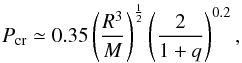 (6)where R and M are given in solar units and Pcr in days. Adopting an estimated radius of the O star in CQ Cep, including uncertainties, in the range 7.7–8.1 R⊙, and q ~ 1, Eq. (6) yields Pcr ~ 1.61−1.71d. Since the CQ Cep orbital period P = 1.64d, a RLO scenario for the O star is clearly feasible. The situation of the WR star is less clear and is discussed below (Sect. 4.1).
We know from Khaliullin (1974) and the use of Eq. (5) that Ṗ< 0 only if the RLO mass donor in the binary system is more massive than its companion. Hence, the alternating sign in Ṗ observed in CQ Cep requires that the sporadic mass transfer leading to Ṗ< 0 originate in the more massive component of the system and be accreted by the less massive one. Unfortunately, the uncertainties in the CQ Cep values of m1 and m2 are too large to be able to establish a priori which of the two stars is the mass donor. Thus, we shall analyze both possibilities2.
We use the stellar parameters from D97, M95, HH97 respectively, which are listed in Table 1. The parameters of D97 and M95 are adopted as representative of cases in which the mass ratio q = MWR/MO9 ≤ 1, while HD97 for the case q> 1.
We consider three scenarios under the Khaliullin et al. (1974) formalism. In Scenario 1 the WR star transfers mass to its O star companion via RLO; that is, the WR star is the RLO donor. In Scenario 2 the O star is the RLO donor with all the transferred mass being accreted by the WR. In Scenario 3 the O star is the RLO donor but a fraction of the transferred matter is carried away by the WR wind. In all cases the WR is the wind-emitting component and we define  yr-1 to be the nominal WR wind value. We assume that the O-star wind is negligible.
In this section, we adopt the usual convention that ṁi< 0 for mass-loss and ṁi> 0 for mass-gain, and that the specific angular momentum is given by  , where ai is the orbital radius of star mi, with i = 1,2. We assign m1 to the WR star and m2 to the O star.
3.1. Scenario 1: WR-star donor
The assumptions in this scenario are: a) The total mass lost from the WR star is ṁ1; b) The amount of mass that is transferred to the O star via RLO is αṁ1, and hence, the stellar wind carries away an amount of mass (1−α)ṁ1; c) The mass that is transferred from the WR to the O star is accreted onto the latter.
The rate at which angular momentum is carried away from the system by the stellar wind is 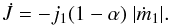 (7)Here we have explicitly included the negative sign due to the mass being lost from m1 (ṁ1< 0) and | ṁ1 | is the absolute value of ṁ1.
Assuming conservative mass-transfer from m1 to m2, the amount of material accreted by m2 is  (8)Substituting conditions (7) and (8) into Eq. (5) yields
 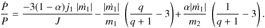 (9)Since we require the binary system to have the ability to display both positive and negative values of Ṗ, the parameter sets of D97 and M95 are excluded, since they correspond to q< 1. We note, however, that with the nominal ṁ1 and no RLO, Eq. (9) yields Ṗ ~ + 0.15 s yr-1 for the D97 and D95 parameter set.
The results for the HH97 parameter set are summarized in Table 3 where the total mass lost from the WR is listed in Col. 2, the amount of wind mass-loss in Col. 3, and the derived value of Ṗ from Eq. (9) in Col. 4. These data show that when the WR wind mass-loss rate is fixed at the nominal value, values of Ṗ from −0.2 to −8.4 s yr-1 are derived, consistent with the range of observed values. These correspond to RLO mass transfer rates in the range (0.8−248) × 10-5M⊙yr-1. There is a problem, however, with the Ṗ> 0 values: In order to derive values consistent with those observed, wind mass-loss rates two to ten times larger than the nominal value are required. Given the uncertainties in the WR mass-loss rates, a factor of two is not significant and could be accomodated using the Hamann & Koesterke (1998) mass-loss rate, but a factor of ten would be difficult to reconcile with determinations based on observations.
In summary, within Scenario 1 the WR can be thought of as occasionally filling and overflowing its Roche lobe, during which time Ṗ< 0 due to accretion onto its lower mass companion. At other times, when Ṗ> 0, the mass loss is dominated by its stellar wind. However, this latter state requires  , values that are between two and ten times larger than the nominal value or an additional process by which angular momentum is removed from the system.
Scenario 1: the WR is the RLO donor.
3.2. Scenario 2: O star donor and conservative mass transfer
In this scenario, the WR star emits a steady wind at the rate  while at the same time it accretes material being transferred through the Roche Lobe by the companion O star. The stellar wind emitted by the WR carries away an amount of angular momentum
  . The mass of m1 is diminished by the wind mass-loss and, at the same time, augmented by the amount of matter it receives from the donor. Thus, in Eq. (5) the term corresponding to
  , where is the wind mass-loss rate and the second term in this sum is equal to the amount of mass transferred from the O star to the WR star. With these considerations, Eq. (5) takes the form,
 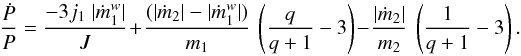 (10)Since the mass donor needs to be more massive than its companion in order to yield Ṗ< 0, the HH97 parameter set is excluded. The results for this scenario are listed in Table 4. Column 1 lists the RLO mass transfer rate and Cols. 2 and 3 list the resulting values of Ṗ for assumed WR wind mass-loss rates 2 × 10⁻⁵M⊙ yr-1 (the nominal value) and three times this value, respectively.
Scenario 2: the O star is the RLO donor.
As in Scenario 1, we find negative values of Ṗ in the range that are observed, but WR mass-loss rates three times the nominal value or larger are needed to obtain Ṗ ≥ 0.4 s yr-1. It is also noteworthy that the accretion rates required to get Ṗ ≃ −8 s yr-1 differ considerably depending on whether the D97 or the M95 parameter sets are used. This is a consequence of the nearly equal masses in the D97 solution.
3.3. Scenario 3: O-star donor and and non-conservative mass transfer
As shown above, both Scenario 1 and Scenario 2 provide an explanation for alternating positive and negative values of Ṗ through the assumption that mass is sporadically transferred by the more massive star and accreted by the less massive one. However, neither scenario can produce the Ṗ ≥ 0.4 s yr-1 values listed in Table 2, even with three times the nominal WR wind mass-loss rate.
One solution to this problem consists of assuming that when the RLO transfer rate is small, the WR wind overcomes the ram pressure of the infalling material and carries this material away from the system. Here we estimate the magnitude of the effect needed. The assumptions are: 1) all of the mass that is lost by the WR leaves the system via the stellar wind; 2) the O star is losing material via RLO; and 3) the WR wind sweeps away this material. Thus, the angular momentum that is lost by the system is 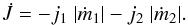 (11)The amount of material lost by m2 is the amount that passes through the inner Lagrangian point L1. It is a variable in our calculation. Hence,
 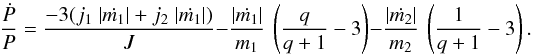 (12)Table 5 illustrates the results from Eq. (12) for the D97 and M95 parameters, where the wind mass-loss rate from the WR star is set at its nominal value. The first column lists the assumed RLO mass-transfer rate from the O star, and the second and third columns list the resulting value of Ṗ from Eq. (12) for the D97 and M95 parameters, respectively. It is interesting to note that relatively small RLO rates (<15 × 10-5M⊙ yr-1) are sufficient to produce positive Ṗ values which are similar to those listed in Table 2. This is consistent with the notion that the WR wind must be able to sweep up the material that is inflowing from L1 and carry it away.
This scenario would hold only until the ram pressure of the inflowing material overcomes that of the WR wind, after which time accretion onto the WR might be expected to occur, leading to the Ṗ< 0 values. The issue of the ram pressure balance is examined in the next section.
Scenario 3: the WR sweeps away O-star material passing through L1.
4. Discussion
Within the standard binary star scenarios, an alternating sign in Ṗ can only occur if, in addition to the wind mass-loss (which leads to Ṗ> 0), mass is sporadically transferred from the more massive star to its companion and accreted by the latter (which leads to Ṗ< 0). Given the uncertainty in the masses of the two stars in CQ Cep, we analyzed the conditions under which an alternating sign in Ṗ would be possible for each of the two cases: the WR star is the donor (Scenario 1) and the O star is the donor (Scenarios 2 and 3). In this section we discuss some of the caveats and possible alternative scenarios.
4.1. Is the WR star the mass donor?
The Ṗ< 0 values under this scenario can only occur if the WR star is the more massive member of the binary system, as in the orbital solution of HH97.
A scenario in which the WR star fills its Roche lobe (Scenario 1) is difficult to sustain assuming that it is an evolved, H-poor WN-type star because the hydrostatic radius of such stars is always much smaller than the extended optically thick wind region above it. For example, the hydrostatic radius of a 20 M⊙ WR star is ~1.2 R⊙ (Schaerer & Maeder 1992). Typically, the wind is already accelerated to a few 100 km s-1 in this region – as is evidenced by the width of the most narrow WR lines, for example, NV 4604 Å (Fig. 5 in Marchenko et al. 1995).
On the other hand, the fact that the O-star absorption lines have not been with high confidence identified, leaves open the possibility that the WR component has unshifted absorption lines, which would be typical of a WN7+abs type, contrary to the case of the H-poor WN6 stars. In this case, the radius of the hydrostatic photosphere would coincide with that deduced from the optical light curves and therefore would be close to the Roche radius. However, Hamann & Koesterke (1998) list CQ Cep with zero hydrogen mass fraction, which would seem to contradict this hypothesis. On the other hand, both these authors and Howarth & Schmutz (1992) give values for the WR stellar radius in the range 9–25 R⊙, well in excess of the Roche radius.
Hence, we cannot exclude the possibility that the WR star is the mass donor, but as mentioned above, this scenario requires the WR wind mass-loss rate to occasionally increase significantly (by factors of approximately eight) to account for the large positive Ṗ values or that an additional mechanism for angular momentum loss from the system be invoked.
4.2. Is the WR star the mass gainer?
In order for the WR star to be the mass gainer (and less massive component of the system) it needs to be able to accrete the material being transferred from the O star. If we only consider the ram pressure balance, a rough estimate can be made in order to determine the feasibility of this scenario.
The ram pressure of a steady WR wind with a mass-loss rate3 and speed vw = vw(r) is 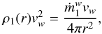 (13)where ρ1(r) is the density of the wind at a distance r from the WR center. The ram pressure of the material streaming from the O star to the WR through L1 is
 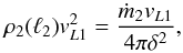 (14)where ℓ2 = a [0.500 + 0.227 log10(m2/m1)] is the approximate distance from m2 to L14, ρ(ℓ2) is the density of the streaming material5, vL1 is the speed with which the streaming material is crossing an area of radius δ centered at L1, and ṁ2 is the corresponding mass-loss rate.
In a classical Roche configuration, the value of δ depends on the degree to which the O star exceeds its Roche lobe, and can conceivably range from δ = 0 when the star just barely touches the Roche lobe to some maximum value δmax which depends on the degree of overcontact. Since there is no observational evidence from CQ Cep to suggest that at any time very large amounts of mass are being lost from the O star, a very large degree of overcontact is not expected. If we assume that the O-star photosphere expands by no more than 5% beyond the L1 point, δmax ~ 3 R⊙.
If accretion is to occur, the ram pressure of the inflowing matter must exceed that of the WR wind, 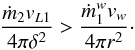 (15)Hence,
  (16)Assuming the nominal value for
  yr-1, vL1 = 2 km s-1 (the approximate thermal speed), r ~ 10 R⊙ (the distance from the center of m1 to L1), this equation can be expressed as
  (17)with δ in solar units and vw in units of 1000 km s-1. Adopting vw = 1300 km s-1 and δ = 0.3 R⊙, Eq. (17) yields ṁ2> 18 × 10-5M⊙ yr-1. This is the minimum RLO mass-transfer rate required for a stream of material of radius 0.3 R⊙ passing through L1 to be able to overcome the WR wind ram pressure.
Let us now consider the constraints imposed on ṁ2 by the positive and negative values of Ṗ listed in Table 2. In order to attain the observed maximum Ṗ ~ + 1 s yr-1, the WR wind should be able to sweep away ~(10−15) × 10-5M⊙ yr-1 (Table 5). Larger mass transfer rates would not be swept away. From Table 4 we see that the Ṗ < 0 values require accretion rates ṁ2 > 40 × 10-5M⊙ yr-1, well above the limit at which the WR wind ram pressure can overcome the inflowing RLO stream.
The inclusion of radiation pressure significantly complicates the assessment, particularly because radiation pressure alters the shape of the gravitational equipotentials from their classical morphology. The classical calculation assumes that the stars are in synchronous rotation and neglects radiation pressure. The consequences of a breakdown in the first of these assumptions is analyzed by Csataryová (1998) and that of the second by Drechsel et al. (1995), and a critical review can be found in Kallrath & Milone (2009). The complexity of the problem implies that further progress requires hydrodynamical calculations of the interaction between the incoming stream and the outgoing WR wind which take into account the radiation pressure from both stars, in addition to all other forces present in the system.
Finally, we note that the hydrodynamics of the interaction also depend on the model that is assumed for the stellar wind. The winds of WR stars are thought to be “clumped” (Puls et al. 2008). The interaction of an incoming stream with the clumps would be highly dependent on the size and density of these inhomogeneities.
4.3. Other scenarios and issues
Other scenarios that could be invoked to produce angular momentum loss from the system include non-conservative mass-loss leading to the formation of a circumbinary disk (Chen et al. 2006) and equatorial ejection of matter from an asynchronously rotating star as a consequence of tidal shear energy dissipation (Koenigsberger & Moreno 2016). Numerical simulations are required, however, in order to determine whether the timescale and magnitude of the instabilities can lead to the observed rates of orbital period change in CQ Cep.
An additional question that is left unanswered refers to the mechanism producing the assumed sporadic expansion of the mass-donor which leads to the Roche lobe overflow. One possibility is that the O star is a low-frequency pulsator. Pulsations associated with WR systems have been reported (Blecha et al. 1992; Baade et al. 1990) but the periods are in the range of seconds to days, which are too small compared to the observed years-timescale in Ṗ variations in CQ Cep. Another possibility is that tidal instabilities may lead to oscillations in the orientation and size of the inner tidal bulge (Moreno & Koenigsberger 1999), especially in eccentric orbits. Although the quoted CQ Cep values e ~ 0.01−0.03 are very small, it only takes a small fluctuation in the tidal deformation to produce an important effect, given the close proximity of the two stars in the system. However, these oscillations occur on orbital timescales and they would not be expected to produce episodic events on timescales of years.
Variations in the O−C diagram on a timescale of years could also be a consequence of the light travel effect (Irwin 1952), if we invoke as an explanation the presence of an as yet unseen third body orbiting the WR+O pair. However, we are unable to ascertain whether the alternating sign in Ṗ that we have found is periodic, and thus we cannot comment further on the possibility of a third component. Given the difficulty in even identifying the spectral signature of the close companion to the WR star, finding evidence for a third object seems challenging. However, it is interesting to note that there is a large dispersion in the systemic velocity (the γ-velocity) that has been derived from radial velocity studies of the N IV 4058 Å emission line. Stickland et al. (1984) provide a summary of these γ-velocities, obtained over ~50 yr of observations and having values from −85 to −55 km s-1 with quoted uncertainties ~1−5 km s-1. If this range in γ-velocities isn’t caused by fluctuations in the WR wind structure, then it could be pointing to the presence of a third body. It is not clear, however, to what extent a third object would induce perturbations in the WR+O orbit since such perturbations are dependent on the assumed mass and orbital parameters of the putative third body (Eggleton & Kiseleva-Eggleton 2001).
5. Conclusions
Stellar wind mass-loss in binary systems carries away angular momentum causing a monotonic increase in the orbital period, Ṗ > 0. Despite possessing a significant stellar wind, the eclipsing Wolf-Rayet binary system CQ Cep does not show the expected monotonic Ṗ increase. In fact, the existing data indicate that on occasions the opposite occurs; that is, Ṗ < 0. In this paper we performed a critical review of the historic records of times of light curve minima in CQ Cep and conclude that Ṗ alternates between positive and negative values on a timescale of years.
Within the standard binary star scenarios, an alternating sign in Ṗ can only occur if, in addition to the wind mass-loss (which leads to Ṗ > 0), mass is sporadically transferred from the more massive star to its companion and accreted by the latter (which leads to Ṗ < 0). We find that the negative values of Ṗ in CQ Cep require sporadic accretion rates in the range (8−248) × 10-5M⊙ yr-1. We also find that occasionally Ṗ exceeds by factors of two to ten that which is predicted for the nominal WR wind mass-loss rate. Assuming that the stellar wind of the O-star companion remains negligible at all times, this implies that either the WR wind mass-loss rate sporadically increases by factors of approximately eight with respect to the nominal value, or that an additional process acts to remove angular momentum from the system.
The large uncertainty in the CQ Cep mass-determinations precludes us from establishing which of the two stars in the system is more massive and thus plays the role of the mass-donor. This issue must be resolved for further progress to be made in understanding the interplay between wind mass-loss and Roche lobe overflow mass transfer. These processes determine the future evolutionary path of both stars in massive binary systems, a path that can lead to a catastrophic merger and/or supernova. Hence, determining the phenomena in play in CQ Cep would be of benefit for understanding binary star interactions and evolutionary processes in general.
Clearly, however, the uncertainties associated with the values of the masses can accomodate a scenario in which both stars are within their RRL.
The discrepancies in derived values of q, resulting largely from claimed detections of photospheric absorption lines arising in the O star, have not been substantiated (see the discussion in HH97). There is also a discrepancy between the photometrically-derived orbital inclination (i ~ 70°) and that which is derived from the polarization measurements (i ~ 82°, HH97). Furthermore, the quoted values for the stellar radii often depend on whether they were derived directly from a fit to the light curve or whether it was assumed that the stars fill their Roche lobes. An extensive discussion of the uncertainties in the stellar radii, effective temperatures and masses is provided by Stickland et al. (1984).
In this subsection, the stated mass loss rates refer to their absolute value.
We note that ℓ2 differs from the Roche radius RRL since the latter is the radius of the sphere that contains the same volume as is contained in the tidally-distorted Roche Lobe.
In a classical Roche configuration, this would be the density of the O star atmosphere layer that extends to L1.
Acknowledgments
G.K. thanks Alex Raga for a helpful discussion, and acknowledges financial support from CONACYT grants 129343 and 252499, UNAM/PAPIIT grant IN 105313, and computer support from Ulises Amaya. We thank an anonymous referee for very helpful comments and suggestions.
References
- Antokhina, E. A., & Cherepashchuk, A. M. 1988, Soviet Astron. Lett., 14, 105 [NASA ADS] [Google Scholar]
- Antokhina, E. A., Lipunova, N. A., & Cherepashchuk, A. M. 1982, Soviet Ast., 26, 429 [NASA ADS] [Google Scholar]
- Baade, D., Schmutz, W., & van Kerkwijk, M. 1990, A&A, 240, 105 [NASA ADS] [Google Scholar]
- Blecha, A., Schaller, G., & Maeder, A. 1992, Nature, 360, 320 [NASA ADS] [CrossRef] [Google Scholar]
- Chen, W.-C., Li, X.-D., & Qian, S.-B. 2006, ApJ, 649, 973 [NASA ADS] [CrossRef] [Google Scholar]
- Cherepashchuk, A. M. 1982, Ap&SS, 86, 299 [NASA ADS] [CrossRef] [Google Scholar]
- Chesneau, O., Meilland, A., Chapellier, E., et al. 2014, A&A, 563, A71 [NASA ADS] [CrossRef] [EDP Sciences] [Google Scholar]
- Chis, G. D., & Pop, V. 1983, in Relativistic Objects in Close Binary Systems, ed. V. Ureche, 152 [Google Scholar]
- Csataryová, M. 1998, in 29th Conf. on Variable Star Research, eds. J. Dusek & M. Zejda, 48 [Google Scholar]
- De Loore, C., & Vanbeveren, D. 1994, A&A, 292, 463 [NASA ADS] [Google Scholar]
- Demircan, O., Ak, H., Ozdemir, S., Tanriver, M., & Albayrak, B. 1997, Astron. Nachr., 318, 267 [NASA ADS] [CrossRef] [Google Scholar]
- Drechsel, H., Haas, S., Lorenz, R., & Gayler, S. 1995, A&A, 294, 723 [NASA ADS] [Google Scholar]
- Eggleton, P. P. 1983, ApJ, 268, 368 [NASA ADS] [CrossRef] [Google Scholar]
- Eggleton, P. 2002, Evolutionary Processes in Binary Stars (Cambridge University Press) [Google Scholar]
- Eggleton, P. P., & Kiseleva-Eggleton, L. 2001, ApJ, 562, 1012 [NASA ADS] [CrossRef] [Google Scholar]
- Gaposchkin, S. 1944, ApJ, 100, 242 [NASA ADS] [CrossRef] [Google Scholar]
- Guseinzade, A. A. 1967, Astrophysics, 3, 160 [NASA ADS] [CrossRef] [Google Scholar]
- Hamann, W.-R., & Koesterke, L. 1998, A&A, 333, 251 [NASA ADS] [Google Scholar]
- Harries, T. J., & Hilditch, R. W. 1997, MNRAS, 291, 544 [NASA ADS] [CrossRef] [Google Scholar]
- Hiltner, W. A. 1950, ApJ, 112, 477 [NASA ADS] [CrossRef] [Google Scholar]
- Howarth, I. D., & Schmutz, W. 1992, A&A, 261, 503 [NASA ADS] [Google Scholar]
- Hurley, J. R., Tout, C. A., & Pols, O. R. 2002, MNRAS, 329, 897 [NASA ADS] [CrossRef] [Google Scholar]
- Irwin, J. B. 1952, ApJ, 116, 211 [NASA ADS] [CrossRef] [Google Scholar]
- Kallrath, J., & Milone, E. F. 2009, Eclipsing Binary Stars: Modeling and Analysis, 2nd edn. (New York: Springer-Verlag) [Google Scholar]
- Kartasheva, T. A. 1972, Peremennye Zvezdy, 18, 459 [NASA ADS] [Google Scholar]
- Kartasheva, T. A. 1976, Soviet Astron. Lett., 2, 197 [NASA ADS] [Google Scholar]
- Khaliullin, K. F. 1974, Soviet Ast., 18, 229 [Google Scholar]
- Koenigsberger, G., & Moreno, E. 2016, Rev. Mex. Astron. Astrofis., 52, 113 [NASA ADS] [Google Scholar]
- Kreiner, J. M., & Tremko, J. 1983, Bull. Astron. Inst. Czechoslovakia, 34, 341 [NASA ADS] [Google Scholar]
- Langer, N. 2012, ARA&A, 50, 107 [NASA ADS] [CrossRef] [Google Scholar]
- Marchenko, S. V., Moffat, A. F. J., Eenens, P. R. J., Hill, G. M., & Grandchamps, A. 1995, ApJ, 450, 811 [NASA ADS] [CrossRef] [Google Scholar]
- Meyer, A. 1972, IBVS, 668 [Google Scholar]
- Moreno, E., & Koenigsberger, G. 1999, Rev. Mex. Astron. Astrofis., 35, 157 [NASA ADS] [Google Scholar]
- Nelson, C. A., & Eggleton, P. P. 2001, ApJ, 552, 664 [NASA ADS] [CrossRef] [Google Scholar]
- Nishimaki, Y., Yamamuro, T., Motohara, K., Miyata, T., & Tanaka, M. 2008, PASJ, 60, 191 [NASA ADS] [CrossRef] [Google Scholar]
- Paczyński, B. 1971, ARA&A, 9, 183 [NASA ADS] [CrossRef] [Google Scholar]
- Paschke, A., & Brat, L. 2006, Open European Journal on Variable Stars, 23, 13 [Google Scholar]
- Podsiadlowski, P., Joss, P. C., & Hsu, J. J. L. 1992, ApJ, 391, 246 [NASA ADS] [CrossRef] [Google Scholar]
- Puls, J., Vink, J. S., & Najarro, F. 2008, A&ARv, 16, 209 [NASA ADS] [CrossRef] [EDP Sciences] [Google Scholar]
- Raucq, F., Rauw, G., Gosset, E., et al. 2016, A&A, 588, A10 [NASA ADS] [CrossRef] [EDP Sciences] [Google Scholar]
- Schaerer, D., & Maeder, A. 1992, A&A, 263, 129 [NASA ADS] [Google Scholar]
- Semeniuk, I. 1968, Acta Astron., 18, 313 [NASA ADS] [Google Scholar]
- Shao, Y., & Li, X.-D. 2016, ApJ, 833, 108 [NASA ADS] [CrossRef] [Google Scholar]
- Skinner, S. L., Zhekov, S. A., Güdel, M., & Schmutz, W. 2015, ApJ, 799, 124 [NASA ADS] [CrossRef] [Google Scholar]
- Smith, N., Gehrz, R. D., Campbell, R., et al. 2011, MNRAS, 418, 1959 [NASA ADS] [CrossRef] [Google Scholar]
- Stickland, D. J., Bromage, G. E., Burton, W. M., et al. 1984, A&A, 134, 45 [NASA ADS] [Google Scholar]
- Tchugainov, P. F. 1960, Peremennye Zvezdy, 13, 148 [NASA ADS] [Google Scholar]
- Vanbeveren, D., van Bever, J., & De Donder, E. 1997, A&A, 317, 487 [NASA ADS] [Google Scholar]
- Walker, E. N., Lloyd, C., Pike, C. D., Stickland, D. J., & Zuiderwijk, E. J. 1983, A&A, 128, 394 [NASA ADS] [Google Scholar]
- Wellstein, S., Langer, N., & Braun, H. 2001, A&A, 369, 939 [NASA ADS] [CrossRef] [EDP Sciences] [Google Scholar]
All Tables
All Figures
|
Fig. 1 The O−C diagram for the primary minima calculated from the linear elements (Eq. (1)). The abscissa is given in units of orbit number, with the origin defined on HJD 2 432 456.671 (1947 Sept. 28) and adopting P0 = 1.64124d. The ordinate is in units of fraction of orbital period. The error bars indicate an assumed precision of ±0.005 in orbital fraction, which corresponds to ~11 min. The red squares denote values from 1947 to 1971 and the blue diamonds denote data from 1971–2014. The last point corresponds to Skinner et al. (2015), who have determined the time of minimum to a precision of 20 s. |
| In the text | |
|
Fig. 2 Same as previous figure only that here we illustrate the quadratic fits to portions of the data that display strong variations. Top: fits with positive quadratic coefficients. Bottom: fits with negative quadratic coefficients. (see Table 2 for the corresponding values). Different symbols indicate the O−C values that were used to derive each parabolic fit reported in Table 1. |
| In the text | |
Current usage metrics show cumulative count of Article Views (full-text article views including HTML views, PDF and ePub downloads, according to the available data) and Abstracts Views on Vision4Press platform.
Data correspond to usage on the plateform after 2015. The current usage metrics is available 48-96 hours after online publication and is updated daily on week days.
Initial download of the metrics may take a while.