| Issue |
A&A
Volume 597, January 2017
|
|
|---|---|---|
| Article Number | L9 | |
| Number of page(s) | 4 | |
| Section | Letters | |
| DOI | https://doi.org/10.1051/0004-6361/201630235 | |
| Published online | 13 January 2017 | |
A non-glitch speed-up event in the Crab Pulsar
No. 24, NTI Layout 1st Stage, 3rd Main, 1st Cross, Nagasettyhalli, 560094 Bangalore, India
e-mail: viv.maddali@gmail.com
Received: 13 December 2016
Accepted: 23 December 2016
Context. The rotation history of the Crab Pulsar is well described by (1) a rotation frequency ν and a slowdown model that is specified by its first two time derivatives  and
and  , known as the secular slowdown model; (2) occasional (once in ≈2 yr) significant and abrupt increases in the magnitude of ν and (occurring on timescales of minutes), known as glitches; and (3) much slower increases and decreases in ν and (occurring over months and years) that are an order of magnitude smaller, known as timing noise.
Aims. This work reports a speed-up event in the Crab Pulsar that occurred around 2015 February that is distinct from glitches and timing noise.
Methods. Monthly νs and s of the Crab Pulsar, obtained at radio frequencies and published by Jodrell Bank Observatory (JBO), are used to demonstrate the speed-up event. Monthly arrival times of the Crab Pulsar’s pulse, also published by JBO, combined with X-ray data from the RXTE, Swift, and NuSTAR observatories are used to verify the result.
Results. The speed-up event is caused by a persistent increase in , which results in a monotonic increase in ν. Over the last ≈550 days, ν has increased monotonically by an amount that is ≈10 times larger than the timing noise level.
Conclusions. This is a unique event in the Crab Pulsar. This is probably due to a small increase in the Crab Pulsar’s internal temperature. In its absence, the next large glitch in the Crab Pulsar is expected to occur around 2019 March. However, this event could have an important bearing on its occurrence.
Key words: pulsars: general / pulsars: individual: Crab Pulsar
© ESO, 2017
1. Introduction
Recently Lyne et al. (2015) discussed the rotation history of the Crab Pulsar over the last 45 yr. By studying the three best (isolated and large) glitches among the 24 that have been observed in the Crab Pulsar so far, they show that the apparently abrupt decrease in at a glitch (increase in magnitude of negative value) actually has a detail: only about half the decrease occurs instantaneously; the rest occurs asymptotically quasi exponentially on a timescale of ≈320 days; see Fig. 3 of Lyne et al. (2015). The three best glitches were chosen by the criteria that a change in the magnitude of ν and at the glitch should be large, and also by the criteria that the previous and subsequent glitches should occur at least 800 days before and 1200 days after each glitch, respectively. However, for the glitch of 2011 November (at MJD 55 875.5; hereafter CPG2011), they only had data for ≈800 days after the glitch, This work analyzes the additional data that has since been published by JBO, which reveals a phenomenon unreported so far in Crab or any other Pulsar.
Figure 1 is similar to panel 3 of Fig. 3 in Lyne et al. (2015). It is obtained from the frequency derivative values tabulated in the so-called Jodrell Bank Crab Pulsar Monthly Ephemeris1 (Lyne et al. 1993; hereafter JBCPME). This paper focuses on the significant departure of the data from the model curve in Fig. 1, starting ≈1200 days after CPG2011 and lasting until now (2016 September 15). This implies a persistent and systematic increase in  with respect to the model of Lyne et al. (2015), which they consider to be the prototypical behavior of all glitches in the Crab Pulsar.
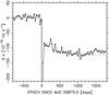 |
Fig. 1 Frequency derivative residual |
Figure 1 is obtained by fitting a straight line to the 28 from JBCPME, as a function of epoch, for the 800 days before CPG2011, resulting in a  value of −370730(2) × 10-15 Hz s-1 at the glitch epoch; the error in the last digit is shown in brackets. The slope
  is 1.182(6) × 10-20 Hz s-2. Subtracting the straight line from the values results in the shown as dots in Fig. 1. The well-studied glitch behavior of the Crab Pulsar implies that the data from days 0 to 1200 should ideally be fit to the model
  (1)the second term representing the longtime recovery proposed by \cite{Lyne2015}in their Eq. (6). Now the short recovery timescale τ1 is typically ≈10 days. However, the JBCPME has only one value within 13 days of CPG2011, and only two values within 34 days of CPG2011, so the cadence of data is too poor to fit to the first term in Eq. (1). Furthermore, the errors on these two are a factor of ≈10 to 30 larger than on the rest of the data. So the data from 100 to 1200 days was fit only to the second term in Eq. (1). The results are
 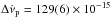 Hz s-1, w = 0.39(3) and τ2 = 510 ± 197 days. By fitting up to 1050 days only, one obtains
 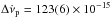 Hz s-1, w = 0.39(5), and τ2 = 367 ± 172 days. These values are consistent with those derived by Lyne et al. (2015), which are
  Hz s-1, w = 0.46, and τ2 = 320 ± 20 days, although the errors on τ2 are very large. In both cases the persistent increase in starting ≈1200 days after CPG2011, of ≈11(1) × 10-15 Hz s-1, is very evident. The dashed curve in Fig. 1 at positive abscissa is obtained using the latter set of parameters.
A persistent increase in should result in a monotonically increasing frequency residual δν, which is the integral of . This is demonstrated in the next section.
2. Analysis of ν
The 28ν values from JBCPME, for the 800 days before CPG2011, were fit to a quadratic curve as a function of epoch. The results are ν0 = 29.706643782(8) Hz at the glitch epoch, the first and second derivatives being 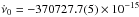 Hz s-1 and
 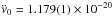 Hz s-2. The last two parameters are statistically consistent with those derived in Sect. 1. Subtracting this quadratic model from the ν data results in the δν shown as dots in the top panel of Fig. 2. The data from 0 to 1200 days were fit to the model
 (2)which is an integral of Eq. (1) with some terms redefined. In both equations the subscripts p and n refer to permanent and exponentially decaying changes, respectively, in the corresponding parameters; see Shemar & Lyne (1996) and Vivekanand (2015) for details. The results for three of the parameters are
 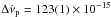 Hz s-1, w = 0.44(2), and τ2 = 317 ± 25 days, which are consistent with the values derived in Sect. 1, and with the values of Lyne et al. (2015). The other three parameters are Δνp = 3.2(2) × 10-7 Hz, Δνn = 12.2(3) × 10-7 Hz, and τ1 = 16 ± 1 days. The step change in ν at CPG2011 is (Δνp + Δνn) × 10+ 7 = 15.4(4) Hz, which compares well with the value of 14.6(1) obtained by Lyne et al. (2015). The step change in at CPG2011 is
  Hz s-1. This number has not been given by Lyne et al. (2015).
Although Eq. (2) is the integration of Eq. (1), two parameters of the latter could only be derived using Eq. (2) for reasons of cadence and large errors. Furthermore, the parameter Δνp is the integration constant that does not exist in Eq. (1).
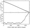 |
Fig. 2 Top panel: frequency residuals δν plotted against epoch since CPG2011. The curve represents the best fit model given in Eq. (2). Bottom panel: difference between the data and the model curve in the top panel. The positive departure of data from the model beyond ≈1200 days is now clearly visible. |
In the top panel of Fig. 2 the model departs from the data from epoch ≈1200 days onwards. This stands out strongly in the bottom panel, which displays the difference between the data and the model. After secular slowdown and glitches have been accounted for in the timing behavior of the Crab Pulsar, one expects to see only timing noise, which is evident before ≈1200 days in the bottom panel. Here δν varies on timescales of ≈100 days with an rms magnitude of ≈1.5 × 10⁻⁸ Hz. However, the speed-up event causes δν to increase monotonically to 47.4 × 10⁻⁸ Hz in ≈550 days. Clearly a monotonic variation that is ≈30 times larger than the rms cannot be due to timing noise. Given the typical monthly cadence of JBCPME data, one can specify the exact epoch of occurrence, and the duration, of this speed-up event only to an accuracy of one month.
Monotonically increasing frequency residuals δν should result in monotonically decreasing residuals of pulse phase, since an increase in frequency leads to a decrease in phase in the TEMPO2 package (see Shemar & Lyne 1996; Vivekanand 2015). This is discussed in the following two sections.
3. Observations of times of arrival
Times of arrival (TOA) of the main peak of the Crab Pulsar are also tabulated in the JBCPME, referred to the solar system barycenter, and scaled to infinite frequency. Eighty-eight of these TOA were combined with TOA from the following three X-ray observatories.
3.1. RXTE observatory
Fifty-seven observation identification numbers (ObsID) are used from the Proportional Counter Array (PCA; Jahoda et al. 1996) of RXTE, the first obtained on 2009 September 12 (ObsID 94802-01-16-00), and the last on 2011 December 31 (ObsID 96802-01-21-00). The data (with event mode identifier E_250us_128M_0_1s) and their analysis are described in detail in Vivekanand (2015, 2016a,b).
3.2. Swift observatory
Forty-four ObsID from the X-Ray Telescope (XRT; Burrows et al. 2005) on board the Swift observatory (Gehrels et al. 2004) were analyzed; data were obtained in the wt mode, which has a time resolution of 1.7791 milliseconds (ms). The first observation was obtained on 2009 September 17 (ObsID 00058990010) and the last on 2016 April 01 (ObsID 00080359006). The TIMEPIXR keyword was set to the value 0.5 (see XRT digest2). The tool xrtpipeline was run with the coordinates of the Crab Pulsar. The rest of the analysis was as described in Vivekanand (2015). The tool barycorr was used for barycentric correction. Pile up in general is not an issue for pulsar timing, since its main effect is to distort the spectrum, and not to affect the arrival times of photons.
3.3. NuSTAR observatory
Thirty-eight ObsID from the NuSTAR observatory (Harrison et al. 2013) were analyzed; they had live times of at least ≈1000 s. The first observation was obtained on 2012 September 20 (ObsID 10013021002) and the last on 2014 October 02 (ObsID 10002001008). The tools nupipeline and barycorr were used. The dead time corrected pulse profile was obtained by using the live time data in the PRIOR column (Madsen et al. 2015). The rest of the analysis was as described in Vivekanand (2015).
4. Analysis of times of arrival
The combined 227 TOA in a duration of ≈1770 days yields a mean cadence of once in ≈8 days, which is a significant improvement over that of JBCPME. All data have been barycenter corrected using the same ephemeris (DE200). The published phase offsets between the X-ray and radio pulses were inserted for the RXTE (Rots et al. 2006) and Swift (Cusumano et al. 2012) observatories. For NuSTAR the measured correction of 5.76 ± 0.13 ms was used, which also includes a UTC clock offset (this issue is currently under discussion with the NuSTAR help desk). The typical rms error on the TOA for the three observatories was 34μs, 136μs, and 750μs, respectively.
Pre-glitch reference timing model obtained using 74 phase residuals ≈500 days before CPG2011, at reference epoch MJD 55 875.5.
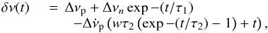
The 74 phase residuals ≈500 days before CPG2011 were fit in TEMPO2 (Hobbs et al. 2006) to obtain the pre-glitch reference timing model (see discussion below), which is given in Table 1; only the last number is not statistically consistent with the values derived in Sect. 2, but it is in the same ballpark. The rms of the fit is 327μs. If the data cadence was sufficient (e.g., once a day), then the TEMPO2 phase residuals for the post-CPG2011 TOA would have been consistent with the integral of the negative of Eq. (2), which is
![\begin{equation} \begin{array}{ll} \delta \phi(t) & \,\,= \,\,\Delta \phi_0 - (1/\nu_0) \left [\Delta \nu_{\rm p} t - \Delta \nu_n \tau_1 \left (\exp-(t/\tau_1) - 1 \right ) \right . \\ &\quad - \left . \Delta \dot \nu_{\rm p} \left ( w \tau_2 \left ( -\tau_2 \left ( \exp-(t/\tau_2) - 1 \right ) - t \right ) + t^2/2 \right ) \right], \\ \end{array} \end{equation}](/articles/aa/full_html/2017/01/aa30235-16/aa30235-16-eq98.png) (3)where δφ is measured in seconds. However, the low data cadence in this work requires that integral number of periods in time (or cycles in phase) must be added or subtracted from the TEMPO2 phase residuals in order to match with Eq. (3). This was done (if required) for each post-glitch residual under the requirements that the modified phase should be as close to Eq. (3) as possible and that the difference between two consecutive modified phases should be less than half a cycle (of either sign), the criterion also used internally in TEMPO2. For this, a special plugin was developed in TEMPO2, which plots Eq. (3) over the data as a guide for inserting the appropriate number of phase cycles. This scheme worked for up to 1450 days after CPG2011, which is sufficient for our purpose. Beyond 1450 days the difference between consecutive phase residuals differs by more than half a cycle.
(3)where δφ is measured in seconds. However, the low data cadence in this work requires that integral number of periods in time (or cycles in phase) must be added or subtracted from the TEMPO2 phase residuals in order to match with Eq. (3). This was done (if required) for each post-glitch residual under the requirements that the modified phase should be as close to Eq. (3) as possible and that the difference between two consecutive modified phases should be less than half a cycle (of either sign), the criterion also used internally in TEMPO2. For this, a special plugin was developed in TEMPO2, which plots Eq. (3) over the data as a guide for inserting the appropriate number of phase cycles. This scheme worked for up to 1450 days after CPG2011, which is sufficient for our purpose. Beyond 1450 days the difference between consecutive phase residuals differs by more than half a cycle.
This technique is merely a modification of the usual method of using TEMPO2, viz., of using the pre-glitch reference timing model on the post-glitch TOAs. If the data cadence was very good, e.g., once a day, then one would have immediately obtained the curve describe by Eq. (3). Given the low data cadence in our data, TEMPO2 has to be aided by manually inserting the integer number of phase cycles (positive or negative) between consecutive phase residuals. This is achieved by using Eq. (3) as a guide.
The top panel of Fig. 3 shows modified phase residuals δφ, after removing a small linear trend from 0 to 1200 days, which implies a small correction of 1.77(1) × 10-8 Hz in period to the reference timing model. This is most probably on account of errors on the parameters of the pre-glitch reference timing model, errors on the parameters of Eq. (3), etc. It is clear that beyond epoch ≈1200 days, the phase reduces monotonically, as expected from Fig. 2.
The reliability of this method is verified in the bottom panel of Fig. 3, which shows the integration of −δν in the bottom panel of Fig. 2, using the Trapezoidal rule, and taking the non-uniform spacing of the data epochs into account. Even though the two curves are expected to be similar, the actual similarity is remarkable.
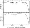 |
Fig. 3 Top panel: phase residuals δφ (in milliseconds) between TOA and Eq. (3), modified as described in the text. The difference between the reference timing models of Sects. 4 and 2 has been taken into account. Bottom panel: integration of the negative of the data in the bottom panel of Fig. 2. |
5. Discussion
In summary, this work has demonstrated that the Crab Pulsar experienced a speed-up event around the end of 2015 February, that was unlike a glitch or a timing noise behavior. It was caused by a persistent increase in of about ≈11(1) × 10-15 Hz s-1 after epoch ≈1200 days from CPG2011. This caused the Crab Pulsar’s ν to increase monotonically by ≈47.4 × 10⁻⁸ Hz over ≈550 days.
In Fig. 3 the pre-glitch reference timing model was obtained using data for the ≈500 days before CPG2011, and not the 800 days that was used in Sects. 1 and 2, because the phase residuals between days 800 and 500 before CPG2011 showed a significant departure from those between days 500 and 0. It is not possible to state here whether this is on account of poor data cadence or on account of a genuine sub-event in the Crab Pulsar.
One physical process that can cause a persistent increase in is an increase in temperature T in the vortex creep regions of the Crab Pulsar (Alpar et al. 1984). Vortex creep is the mechanism by which superfluid vortexes move radially outwards steadily, thus slowing down the superfluid and speeding up the outer crust, to which the radiation that we observe is firmly anchored. Vortexes move radially outwards at speed Vr, which is a statistical quantity, having both signs in general. However, owing to differential rotation between the inner superfluid and the outer crust of a neutron star, it is biased towards positive values. Thus its average value ⟨Vr⟩ is greater than 0, and depends exponentially upon the T. A change in temperature δT gives rise to a change in ⟨Vr⟩, which in turn gives rise to a change in according to the formula  (4)see Eqs. (65) and (22) in Alpar et al. (1984). Strictly, Vr is related to
  , where νs is the frequency of rotation of the superfluid (Eq. (4) in Alpar et al. 1984); νs is related to the observed ν through Eq. (19) of Alpar et al. (1984).
Now, the at epoch ≈1200 days after CPG2011 is equal to  Hz s-1, from Fig. 1, while the persistent increase in this quantity is 11(1) × 10-15 Hz s-1. Therefore,
  is ≈11/370853 ≈ 3.0(3) × 10-5. Thus, the required change in temperature is δT/T ≈ 10-6, which appears to be a very small quantity. Then why are speed-up events so rare in the Crab Pulsar?
The first reason is that the required change in temperature in Eq. (4) may be an underestimate. It is obtained by Alpar et al. (1984) by ignoring the second term in their Eq. (16), which may modify the dependence of on δT in Eq. (4).
The second reason is given in the paragraph following Eq. (65) of Alpar et al. (1984). The heat capacity and thermal conductivity of relativistic electrons give a very small thermal diffusion timescale of about 1 s over 100 m (Flowers & Itoh 1976). Therefore, any heat creating process may not succeed in raising the temperature uniformly and persistently over a sufficiently large creep region, due to rapid dissipation of heat to neighboring regions.
What is the cause of the sudden increase in temperature in the regions of vortex creep? It could be some fluctuation in the vortex creep process itself, since this process can generate significant heat (Alpar et al. 1984). This fluctuation could be due to either magnetic reconnection or relatively slow crustal failure that does not lead to a glitch.
This speed-up event has important implications for the next large glitch in the Crab Pulsar. Glitches are supposed to occur when superfluid vortexes unpin catastrophically, which occurs when the differential rotation between the pinned internal superfluid and outer crust builds up to a critical value (Eq. (11) in Alpar et al. 1984). Clearly, a speed-up event reduces differential rotation; angular momentum is transferred fromthe faster rotating superfluid to the slower crust, which should work against the occurrence of (at least) a large glitch. Therefore, one should logically expect this speed-up event to be terminated well before the next large glitch in the Crab Pulsar. On the other hand, perhaps the magnitude of the speed-up event is so small that the differential rotation may continue to build up to its critical value, but more slowly, so the next large glitch in the Crab Pulsar may occur much later than expected. Therefore, whether the speed-up event persists at the time of the next glitch or is terminated before the next glitch – and if terminated then before what duration – is an important clue to understanding the superfluid dynamics of the Crab Pulsar.
When is the next large glitch expected to occur in the Crab Pulsar? By analyzing the epochs of occurrence of the 24 glitches listed in Table 3 in Lyne et al. (2015), and including the glitch at epoch ≈44 900 listed in Table 3 in Wong et al. (2001), one finds a periodicity of ≈2686 ± 161 days (≈7.4 yr) for the occurrence of glitches in the Crab Pulsar, buried in what otherwise appears to be random occurrence. In particular, all large glitches, defined by Δν/ν> 30 × 10-9 in Table 3 in Lyne et al. (2015), occur at epochs that are at intervals of ≈2686 ± 161 days, or multiples of it, from MJD 42 447.26 (1975 February), which is the epoch of occurrence of the first recorded large glitch in the Crab Pulsar. If one assumes that these statistics are stationary, and that the era of frequent glitching in the Crab Pulsar is over, as is apparent from the data, and that the speed-up event has a negligible effect on the statistics, then the next large glitch in the Crab Pulsar is expected to occur ≈2686 days after the last large glitch, which would imply around MJD 55 875.5 + 2686 ≈ 58 561, or around 2019 late March, with an rms uncertainty of ≈161 days. Whether this glitch will be large or small, and how much later or earlier than 2019 late March it will occur, will be determined by the effect of the speed-up event on achieving critical differential rotation.
Acknowledgments
I thank Sergio Campana for detailed help in enhancing the clarity of and shortening this paper. This research made use of data obtained from the High Energy Astrophysics Science Archive Research Center Online Service, provided by the NASA-Goddard Space Flight Center.
References
- Alpar, M. A., Anderson, P. W., Pines, D., & Shaham, J. 1984, ApJ, 276, 325 [NASA ADS] [CrossRef] [Google Scholar]
- Burrows, D. N., Hill, J. E., Nousek, J. A., et al. 2005, Space Sci. Rev., 120, 165 [NASA ADS] [CrossRef] [Google Scholar]
- Cusumano, G., La Parola, V., Capalbi, M., et al. 2012, A&A, 548, A28 [NASA ADS] [CrossRef] [EDP Sciences] [Google Scholar]
- Flowers, E., & Itoh, N. 1976, ApJ, 206, 281 [NASA ADS] [Google Scholar]
- Gehrels, N., Chincarini, G., Giommi, P., et al. 2004, ApJ, 611, 1005 [NASA ADS] [CrossRef] [Google Scholar]
- Harrison, F. A., Craig, W. W., & Christensen, F. E., et al. 2013, ApJ, 770, 103 [NASA ADS] [CrossRef] [Google Scholar]
- Hobbs, G. B., Edwards, R. T., & Manchester, R. N. 2006, MNRAS, 369, 655 [NASA ADS] [CrossRef] [Google Scholar]
- Jahoda, K., Swank, J. H., Giles, A. B., et al. 1996, Proc. SPIE, 2808, 59 [NASA ADS] [CrossRef] [Google Scholar]
- Lyne, A. G., Pritchard, R. S., & Graham Smith, F. 1993, MNRAS, 265, 1003 [NASA ADS] [CrossRef] [Google Scholar]
- Lyne, A. G., Jordan, C. A., Graham-Smith, F., et al. 2015, MNRAS, 446, 857 [NASA ADS] [CrossRef] [Google Scholar]
- Madsen, K. K., Reynolds, S., Harrison, F., et al. 2015, ApJ, 801, 66 [NASA ADS] [CrossRef] [Google Scholar]
- Rots, A. H., Jahoda, K., & Lyne, A. G. 2004, ApJ, 605, L129 [NASA ADS] [CrossRef] [Google Scholar]
- Shemar, S. L., & Lyne, A. G. 1996, MNRAS, 282, 677 [NASA ADS] [CrossRef] [Google Scholar]
- Vivekanand, M. 2015, ApJ, 806, 190 [NASA ADS] [CrossRef] [Google Scholar]
- Vivekanand, M. 2016a, A&A, 586, A53 [NASA ADS] [CrossRef] [EDP Sciences] [Google Scholar]
- Vivekanand, M. 2016b, ApJ, 826, 187 [NASA ADS] [CrossRef] [Google Scholar]
- Wong, T., Backer, D. C., & Lyne, A. G. 2001, ApJ, 548, 447 [NASA ADS] [CrossRef] [Google Scholar]
All Tables
Pre-glitch reference timing model obtained using 74 phase residuals ≈500 days before CPG2011, at reference epoch MJD 55 875.5.
All Figures
|
Fig. 1 Frequency derivative residual |
| In the text | |
|
Fig. 2 Top panel: frequency residuals δν plotted against epoch since CPG2011. The curve represents the best fit model given in Eq. (2). Bottom panel: difference between the data and the model curve in the top panel. The positive departure of data from the model beyond ≈1200 days is now clearly visible. |
| In the text | |
|
Fig. 3 Top panel: phase residuals δφ (in milliseconds) between TOA and Eq. (3), modified as described in the text. The difference between the reference timing models of Sects. 4 and 2 has been taken into account. Bottom panel: integration of the negative of the data in the bottom panel of Fig. 2. |
| In the text | |
Current usage metrics show cumulative count of Article Views (full-text article views including HTML views, PDF and ePub downloads, according to the available data) and Abstracts Views on Vision4Press platform.
Data correspond to usage on the plateform after 2015. The current usage metrics is available 48-96 hours after online publication and is updated daily on week days.
Initial download of the metrics may take a while.