| Issue |
A&A
Volume 598, February 2017
|
|
|---|---|---|
| Article Number | A106 | |
| Number of page(s) | 6 | |
| Section | The Sun | |
| DOI | https://doi.org/10.1051/0004-6361/201629717 | |
| Published online | 08 February 2017 | |
Temperature dependent growth rates of the upper-hybrid waves and solar radio zebra patterns
1 Department of Theoretical Physics and Astrophysics, Masaryk University, Kotlářská 2, 611 37 Brno, Czech Republic
e-mail: jbenacek@physics.muni.cz
2 Astronomical Institute of the Czech Academy of Sciences, Fričova 258, 251 65 Ondřejov, Czech Republic
3 St.-Petersburg State University, 198504 St.-Petersburg, Russia
Received: 14 September 2016
Accepted: 24 November 2016
Context. The zebra patterns observed in solar radio emission are very important for flare plasma diagnostics. The most promising model of these patterns is based on double plasma resonance instability, which generates upper-hybrid waves, which can be then transformed into the zebra emission.
Aims. We aim to study in detail the double plasma resonance instability of hot electrons, together with a much denser thermal background plasma. In particular, we analyse how the growth rate of the instability depends on the temperature of both the hot plasma and background plasma components.
Methods. We numerically integrated the analysed model equations, using Python and Wolfram Mathematica.
Results. We found that the growth-rate maxima of the upper-hybrid waves for non-zero temperatures of both the hot and background plasma are shifted towards lower frequencies comparing to the zero temperature case. This shift increases with an increase of the harmonic number s of the electron cyclotron frequency and temperatures of both hot and background plasma components. We show how this shift changes values of the magnetic field strength estimated from observed zebras. We confirmed that for a relatively low hot electron temperature, the dependence of growth rate vs. both the ratio of the electron plasma and electron cyclotron frequencies expresse distinct peaks, and by increasing this temperature these peaks become smoothed. We found that in some cases, the values of wave number vector components for the upper-hybrid wave for the maximal growth rate strongly deviate from their analytical estimations. We confirmed the validity of the assumptions used when deriving model equations.
Key words: Sun: radio radiation / instabilities / methods: analytical
© ESO, 2017
1. Introduction
Zebra patterns (zebras) are fine IV radio-burst type structures, observed during solar flares in the dm- and m-wavelength ranges (Slottje 1972; Chernov et al. 2012). They are considered to be an important source of information about the plasma density and intensity of the magnetic field in their sources.
There are many zebra models (Rosenberg 1972; Kuijpers 1975; Zheleznyakov & Zlotnik 1975; Chernov 1976, 1990; LaBelle et al. 2003; Kuznetsov & Tsap 2007; Bárta & Karlický 2006; Ledenev et al. 2006; Laptukhov & Chernov 2009; Tan 2010; Karlický 2013). The most promising one is based on the double plasma resonance instability of the plasma, together with loss-cone type electron distribution function (Zheleznyakov & Zlotnik 1975; Zlotnik 2013). In this model, the upper-hybrid waves are first generated, then transformed to electromagnetic (radio) waves with the same (fundamental branch) or double frequency (harmonic branch) as the upper-hybrid waves. This model has the simple resonance condition (1)where
  is the upper-hybrid frequency of the background plasma, ωp and ωB are electron-plasma and electron-cyclotron frequencies and s is a integer harmonic number, is used for estimations of the magnetic field strength and electron plasma density in zebra radio sources (Ledenev et al. 2001; Zlotnik 2013; Karlický & Yasnov 2015). However, this resonance condition is only valid in the zero-temperature limit. If we want to analyse effects of temperatures on the zebra generation processes, we need to take the resonance condition in its general form, see relation 3.
In this paper we study these temperature effects in detail. It is shown that these effects require a correction in the method used to estimate magnetic field strength in zebra radio sources, especially for zebra stripes at high harmonics.
The paper is structured as follows: in Sect. 2 we present model equations describing the double plasma resonance instability and methods of their solution. Results are summarized in Sect. 3. Finally, the paper is completed by discussions and conclusions in Sects. 4 and 5.
2. Model
Similarly to Winglee & Dulk (1986), Yasnov & Karlický (2004), for the hot electron component we consider the DGH distribution function with the parameter j = 1 (Dory et al. 1965)  (2)where u⊥ = p⊥/me and u∥ = p∥/me are electron velocities and p⊥ and p∥ are components of the electron momentum perpendicular and parallel to the magnetic field, and me is the electron mass. For simplification and in agreement with Winglee & Dulk (1986), we call vt here the thermal velocity of hot electrons and we use the term the temperature of hot electrons, although the distribution function in relation 2 is not Maxwellian.
Unlike Winglee & Dulk (1986), we included the background plasma with non-zero temperature. Its density nb is assumed to be much greater than the density of the hot electrons nh.
In agreement with the approach by Melrose & Dulk (1982), Winglee & Dulk (1986), Yasnov & Karlický (2004), we use the condition for double plasma resonance instability in the form  (3)where
  is the upper-hybrid frequency of the background plasma, where the temperature effect is included, vtb is the thermal velocity of the background plasma,
  is the Lorentz factor, k is the absolute value of the wave number vector. Its componets k∥ and k⊥ are in parallel and perpendicular directions to the magnetic field.
Then, starting from the basic equations presented in Winglee & Dulk (1986), Yasnov & Karlický (2004), we derived the relation for the growth rate ΓUH of the upper-hybrid waves as
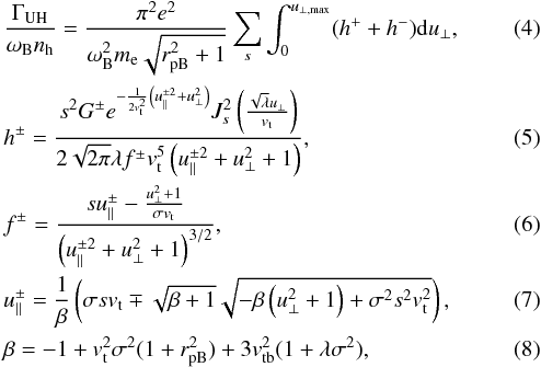
where nh is the hot electron density, e is the electron charge, rpB is the ratio ωp/ωB, Js(x) is the Bessel function of first kind of sth order and λ,σ are dimensionless parameters 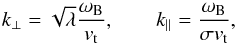 (9)and G± are functions
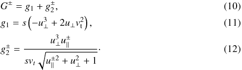 The term
  comes from original relation of derivation distribution function of hot electrons (k∥u⊥∂f/∂u∥) /γ (Winglee & Dulk 1986, Eq. (A8)). As shown below, this term is negligible, and thus in our computations we use G± = g1.
The sum h+ + h− expresses a simultaneous effect of the both operators h+,h− on one upper-hybrid wave described by the specific k-vector. In our computations we used both operators, but we found that term h− was always at least two orders lower than h+ and the typical difference was ten orders.
Equations (4)–(8)are valid for k⊥ ≫ k∥, see Winglee & Dulk (1986). We note that comparing these relations with those in the paper by Yasnov & Karlický (2004) the growth rate (relation 5, G± = g1) is proportional to s3, not to s2.
The integration is done for velocities up to their maxima 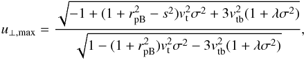 (13)from which we get the followning conditions for maximal and minimal value of λ and σ (expressions under root in previous equations equal zero):
For the comparison below, we add values of σ and λ for the maximal growth rate as follows from analytical estimations made by Winglee & Dulk (1986)

2.1. Methods
We used Python SympPy1 library for analytical application and Python SciPy2 library for numerical computations of growth rate Eqs. (4)–(8), (13)–(16).
Generally, the analytical expressions for the growth rate (relations 4–8) depend on vt, vtb, λ, σ, s and rpB. Their numerical solutions are made in several steps as described below.
First of all is the choice of thermal velocities vt, vtb. Then we selected the rpB interval in which computations are made and steps in this interval. We usually use the interval rpB = 3−20 with the step as ΔrpB = 0.03.
For each value of rpB we searched for s which fulfill s = s0−m,...,s0 + n, where s0 = Round(rpB) is the round value of rpB. Numbers m,n ∈N creates the interval of s for which the growth rate can be computed. However, we limited this interval only for s, maximal values of the growth rate of this interval are at least one hundredth of the maximal growth rate for s0.
Next, values of vt, vtb, rpB and s were chosen, and values of remaining variables λ and σ, which correspond to the k-vector components of the upper-hybrid waves, need to be specified. We chose these values in the intervals σ ∈ (σmin,σmax) and λ ∈ (λmin,λmax) on equidistant lattice. If the maximal values of σmax and λmax are too large or not defined, the upper boundaries are chosen as ten times of their minimal values. It was found to be sufficient in all cases.
Only then it is possible to compute the growth rate given by relations between four and eight for parameters vt, vtb and rpB for each s and in all points of the map λ−σ. In following step we summed the maps in each specific (λ−σ)-point over s. Finally, in the resulting map we searched for the point (λΓmax,σΓmax), where is the highest value of the growth rate, which is then that determined for chosen rpB. The wave number components of the upper-hybrid wave with the maximal growth rate is then determined by Eq. (9).
3. Results
We solved the above described equations for the parameters shown in Table 1, for rpB = 3−20 and B = 100 G. In Models 1−3, we changed background temperature while temperature of the hot electrons remains constant. Models 4 and 5 consider higher temperatures of the hot electrons comparing with Model 1, while the temperature of the background plasma is fixed.
Computation parameters.
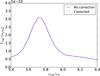 |
Fig. 1 Example of the comparison of the growth rates computed with and without the term |
First, we tested an importance of the correction term  in Eq. (10)for computation of the growth rate. An example of such comparison is shown in Fig. 1. We found that in all models differences in values of the growth rate in models with and without this term is less than 5%, and at their maxima even smaller. Thus, we consider the effect of this term negligible and in all following computations we suppose
  .
.
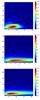 |
Fig. 2 Growth rates in the λ−σ space: Model 1 (top), Model 4 (middle), Model 5 (bottom); all computed for s = 6 and rpb, for which the growth rate is maximal. In Model 1 rpb = 5.8, compare with Fig. 3. Black diamonds show positions of maximal values of the growth rate. |
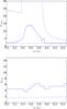 |
Fig. 3 Values of σ (top) and λ (bottom) for Model 1 and s = 6, where the growth rate has the maximal value depending on rpB. Solid lines show values of the maximal growth rate, dash-dotted lines are boundaries of the σ−λ space. Where dash-dotted lines are not shown, the boundaries are outside the presented region. |
In computations of the growth rate in all models (see Table 1) we followed steps described in Methods. Thus, we obtained many maps in the λ−σ space, corresponding to the k-vector space. We note that the relations between the λ−σ and k-vector space is given by relation 9.
Examples of such maps for s = 6 at their maxima are shown in Fig. 2. In each of these maps the maximal growth rate is indicated. Then we summed the maps over s and in the resulting map we searched for the maximal growth rate. This growth rate then corresponds to one point of the curve in Fig. 4.
To compare the computed and analytically estimated (relations 17–18) k-vectors, which correspond to the maximal growth rate for the cases presented in Fig. 2, these are shown in Table 2. Thus, the assumption (k⊥ ≫ k∥) used in derivation of the growth-rate relations was fulfilled in all studied Models. All computed k-vectors are smaller than that analytically predicted. Their computed perpendicular components are systematically two times less than analytical ones. This is due to assumptions and simplifications made in analytical estimations of these values. Computed values of k∥ decrease with increasing temperature in contradiction with analytical predictions.
Examples of values σΓ,max,λΓ,max for vt = 0.1 c (Model 1), where the growth rate has the maximal value depending on rpb, are presented in Fig. 3. Values of σΓ,max for rpB ~ 5 and rpB > 6 are close to the lower boundary (given by Eq. (15)). However, in the region around the growth-rate maximum they deviate from the lower boundary. Values of λΓ,max are changing only slightly. The steps in curves are due to discretisation of the λ−σ space. Note that the value λΓ,max ≈ 5 (Fig. 3, bottom) is less then predicted value s2/ 2 = 18.
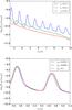 |
Fig. 4 Growth rates in Models shown in Table 1 in dependence on rpB = ωp/ωB. Upper part: growth rates for Models 1, 4 and 5 with the fixed background temperature vtb = 0.018c. Bottom part: growth rates for Models 1–3 with the fixed temperature of hot electrons vt = 0.1c; detailed view. |
Based on many such λ−σ maps the growth-rate in dependence on the rpB = ωp/ωB were computed for all Models according to Table 1. These growth rates are shown in Fig. 4. The upper part of this figure shows an effect of the temperature increase of the hot electrons for fixed temperature of the background plasma electrons, and its bottom part an effect of the temperature increase of the background plasma electrons for fixed temperature of hot electrons.
As seen in the upper part of this figure, Model 1 with the lower velocity of hot electrons have higher growth rates than those in Models 4 and 5 for all rpB = ωp/ωB. Furthermore, the temperature increase of hot electrons smooths peak maxima in the growth rate. While Model 1 shows distinct maxima, in Model 5 the maxima for s> 5 are hardly recognisable.
On the other hand, the change of the thermal velocity of background electrons in Models 1–3 for fixed temperature of hot electrons (see the bottom part of the Fig. 4) do not change values of the growth rate, but the temperature increase shifts the maxima slightly to lower rpB. The values of maxima generally decrease with an increase of rpB.
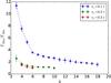 |
Fig. 5 Ratio between maxima and minima of growth rate depending on s for Models 1, 4 and 5. |
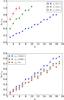 |
Fig. 6 Relative frequency shift Δω of growth-rate maxima between predicted values by ωUH = sωB and its computed position (see Fig. 4). Top: Models 1, 4 and 5 with changing hot electrons temperature; bottom: Models 1–3 with changing background temperature. |
As already mentioned, maxima of the growth rates are more distinct for lower temperatures of the hot electrons. Therefore in Fig. 5 we present ratios of these maxima and neighbouring minima of the growth rate in dependence on s. We note that there is a simple relation between s and rpB;  . As seen in Fig. 5, the ratios decrease with increasing s. It does not depend on the temperature of background electrons.
There is another interesting effect of temperatures of the both hot and background plasma electrons. Namely, by increasing these temperatures, the growth-rate maxima are shifted to lower frequencies as shown in Fig. 6.
In Fig. 7 we present this effect in a way that is more appropriate for zebra pattern analysis. Here we show growth-rate dependence on the ratio ωUH/ωB = s for Model 1, meaning that, with the magnetic field intensity B = 100 G (fB = ωB/ 2π= 280 MHz) and for the model with similar parameters as in Model 1, except that the magnetic field intensity is B = 10 G (fB = ωB/ 2π= 28 MHz). At the horizontal axis of this figure we used the ratio ωUH/ωB, because ωUH can be directly determined from frequencies of the observed zebra stripes. As shown here, the growth-rate maxima do not correspond to a simple resonance conditions (relation 1), which is used in estimations of the magnetic field and plasma density in the zebra radio sources from observed zebras. The maxima are shifted to lower frequencies, and this shift increases with the increase of s. Moreover, as seen in Fig. 7, the relative bandwidth of the growth-rate maxima also increases with the increase of s.
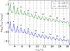 |
Fig. 7 Growth rate for Model 1 (B = 100 G, fB = ωB/ 2π= 280 MHz) (blue line) and the model with similar parameters to Model 1, except the magnetic field intensity B = 10 G (fB = ωB/ 2π= 28 MHz) in dependence on ωUH/ωB. Numbers close the growth-rate maxima designate s from computations. We note that the growth rate at this figure is normalized by the term nhωB. |
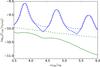 |
Fig. 8 Comparison of the growth rates with summation over s and for s with the maximal growth rate, for Model 1 (blue line) and Model 5 (green line). Dashed lines show summation over s and solid lines correspond to s with the maximal growth rate. |
We also analyzed an effect of summation over s in relation 4 in comparison with the case for s with the maximal growth rate, see Fig. 8 made for Models 1 and 5. As seen here, for lower temperatures vt the summation increases values of the growth-rate minima and for higher temperatures the growth rate is enhanced in the whole range. We found that if for a given s the growth rate decreases steeply from its maximum (the case with lower vt), the summation is important at places where the individual orders overlap. But if the decrease of the growth rate from its maximum is gradual (the case with higher vt), the summation influences the growth rate in a broad range of rpB.
4. Discussion
In the present paper we studied effects of non-zero temperatures of the both hot and background plasma on the growth rate. We showed that including effects of non-zero temperatures leads to shifts in the growth-rate maxima to lower frequencies, comparing frequencies derived from the simple resonance condition ωUH = sωB. We found that these shifts are greater for higher values of the cyclotron harmonic number s. Because the simple resonance condition is used in estimations of the magnetic field and plasma density in the zebra radio sources, these shifts influence such estimations.
Therefore, let us estimate an error in the magnetic field determination from some zebra stripes using the simple resonance condition. For this purpose, let us assume the zebra stripe on the frequency f = fUH = ωUH/ 2π= 504 MHz (assuming the emission on the fundamental frequency) with s= 18. If we use the simple resonance condition then for such high s the ratio of rpB = ωp/ωB≈s, and thus fB = ωB/ 2π= 28 MHz, which gives the magnetic field B= 10 G, see also Fig. 7. But, for modified Model 1 with B= 10 G we found that the emission maximum for s= 18 is shifted to ωUH/ωB= 17.3. From observations, we have fUH = ωUH/ 2π= 504 MHz, thus fB = 504/17.3≈ 29.1 MHz, which gives the magnetic field B= 10.4 G. This example shows a 4% error in magnetic field estimation. As shown in Fig. 6, the shift of the growth rates grows linearly with s. However, the relative error of determining the magnetic field does not depend on s. For higher temperatures of hot electrons errors in magnetic field estimations are larger. For example, for Model 4 (recognisable maxima only for s< 11) this error is ≈16%.
The growth rate is proportional to the density of the hot plasma nh and inversely proportional to the magnetic field. If we multiply the growth rate for Model 3 (with zero temperature of the background plasma), expressed in our paper as ΓUH/ (ωBnh) by the density nh = 108 cm-3 we obtain the growth rate, which agrees with that by (Winglee & Dulk 1986).
In agreement with the results by Yasnov & Karlický (2004) we found that for a relatively low temperature of the hot electrons (Model 1) the dependence of the growth rate vs. the ratio of the electron plasma and electron cyclotron frequencies expresses distinct peaks and increasing this temperature (Models 4 and 5) these peaks are smoothed, especially for high s. This growth-rate behaviour differs from those in previous studies (Zheleznyakov & Zlotnik 1975; Winglee & Dulk 1986). The difference is caused by relativistic corrections used in the present
paper in both resonance terms in Eq. (3)and in selection of maximal growth rates in k-maps. We note that a similar effect in growth-rate behaviour was found by Kuznetsov & Tsap (2007). Namely, considering the power-law and loss-cone distribution function of hot electrons, they showed that stripes of a zebra pattern become more pronounced with an increase of the loss-cone opening angle and the power-law spectral index.
We also studied effects of the neglected term in the growth rate with  (Winglee & Dulk 1986, Eq. (A8)). We found that these effects are negligible.
5. Conclusions
We found that the growth-rate maxima of the upper-hybrid waves for non-zero temperatures of the both hot and background plasma are shifted towards lower frequencies comparing to the zero temperature case. It was found that this shift increases with an increase of the harmonic number s of the electron cyclotron frequency and temperatures of the both hot and background plasma components.
We showed that this shift of the growth-rate maxima influences estimations of the magnetic field strength in sources of observed zebras. In agreement with previous studies we found that for a relatively low temperature of the hot electrons the dependence of the growth rate vs. the ratio of the electron plasma and electron cyclotron frequencies expresses distinct peaks and increasing this temperature these peaks are smoothed.
We found that in some cases the values of components of the wave number vector of the upper-hybrid wave for the maximal growth rate strongly deviate from their analytical estimations. Validity of the assumptions used in derivation of the model equations was confirmed.
Acknowledgments
The authors thank G. P. Chernov for useful comments. We acknowledge support from Grants P209/12/0103. Access to computing and storage facilities owned by parties and projects contributing to the National Grid Infrastructure MetaCentrum provided under the programme “Projects of Projects of Large Research, Development, and Innovations Infrastructures” (CESNET LM2015042), is greatly appreciated. L.Y. acknowledges support by the RFBR grant (No. 16-02-00254).
References
- Bárta, M., & Karlický, M. 2006, A&A, 450, 359 [NASA ADS] [CrossRef] [EDP Sciences] [Google Scholar]
- Chernov, G. P. 1976, Sov. Astron., 20, 449 [Google Scholar]
- Chernov, G. P. 1990, Sol. Phys., 130, 75 [NASA ADS] [CrossRef] [Google Scholar]
- Chernov, G. P., Sych, R. A., Meshalkina, N. S., Yan, Y., & Tan, C. 2012, A&A, 538, A53 [NASA ADS] [CrossRef] [EDP Sciences] [Google Scholar]
- Dory, R. A., Guest, G. E., & Harris, E. G. 1965, Phys. Rev. Lett., 14, 131 [NASA ADS] [CrossRef] [Google Scholar]
- Karlický, M. 2013, A&A, 552, A90 [NASA ADS] [CrossRef] [EDP Sciences] [Google Scholar]
- Karlický, M., & Yasnov, L. V. 2015, A&A, 581, A115 [NASA ADS] [CrossRef] [EDP Sciences] [Google Scholar]
- Kuijpers, J. M. E. 1975, Ph.D. Thesis, Utrecht, Rijksuniversiteit, 72 [Google Scholar]
- Kuznetsov, A. A., & Tsap, Y. T. 2007, Sol. Phys., 241, 127 [NASA ADS] [CrossRef] [Google Scholar]
- LaBelle, J., Treumann, R. A., Yoon, P. H., & Karlický, M. 2003, ApJ, 593, 1195 [NASA ADS] [CrossRef] [Google Scholar]
- Laptukhov, A. I., & Chernov, G. P. 2009, Plasma Phys. Reports, 35, 160 [NASA ADS] [CrossRef] [Google Scholar]
- Ledenev, V. G., Karlický, M., Yan, Y., & Fu, Q. 2001, Sol. Phys., 202, 71 [NASA ADS] [CrossRef] [Google Scholar]
- Ledenev, V. G., Yan, Y., & Fu, Q. 2006, Sol. Phys., 233, 129 [NASA ADS] [CrossRef] [Google Scholar]
- Melrose, D. B., & Dulk, G. A. 1982, ApJ, 259, 844 [NASA ADS] [CrossRef] [Google Scholar]
- Rosenberg, H. 1972, Sol. Phys., 25, 188 [NASA ADS] [CrossRef] [Google Scholar]
- Slottje, C. 1972, Sol. Phys., 25, 210 [NASA ADS] [CrossRef] [Google Scholar]
- Tan, B. 2010, Astrophys. Space Sci., 325, 251 [NASA ADS] [CrossRef] [Google Scholar]
- Winglee, R. M., & Dulk, G. A. 1986, ApJ, 307, 808 [NASA ADS] [CrossRef] [Google Scholar]
- Yasnov, L. V., & Karlický, M. 2004, Sol. Phys., 219, 289 [NASA ADS] [CrossRef] [Google Scholar]
- Zheleznyakov, V. V., & Zlotnik, E. Y. 1975, Sol. Phys., 44, 461 [NASA ADS] [CrossRef] [Google Scholar]
- Zlotnik, E. Y. 2013, Sol. Phys., 284, 579 [NASA ADS] [CrossRef] [Google Scholar]
All Tables
All Figures
|
Fig. 1 Example of the comparison of the growth rates computed with and without the term |
| In the text | |
|
Fig. 2 Growth rates in the λ−σ space: Model 1 (top), Model 4 (middle), Model 5 (bottom); all computed for s = 6 and rpb, for which the growth rate is maximal. In Model 1 rpb = 5.8, compare with Fig. 3. Black diamonds show positions of maximal values of the growth rate. |
| In the text | |
|
Fig. 3 Values of σ (top) and λ (bottom) for Model 1 and s = 6, where the growth rate has the maximal value depending on rpB. Solid lines show values of the maximal growth rate, dash-dotted lines are boundaries of the σ−λ space. Where dash-dotted lines are not shown, the boundaries are outside the presented region. |
| In the text | |
|
Fig. 4 Growth rates in Models shown in Table 1 in dependence on rpB = ωp/ωB. Upper part: growth rates for Models 1, 4 and 5 with the fixed background temperature vtb = 0.018c. Bottom part: growth rates for Models 1–3 with the fixed temperature of hot electrons vt = 0.1c; detailed view. |
| In the text | |
|
Fig. 5 Ratio between maxima and minima of growth rate depending on s for Models 1, 4 and 5. |
| In the text | |
|
Fig. 6 Relative frequency shift Δω of growth-rate maxima between predicted values by ωUH = sωB and its computed position (see Fig. 4). Top: Models 1, 4 and 5 with changing hot electrons temperature; bottom: Models 1–3 with changing background temperature. |
| In the text | |
|
Fig. 7 Growth rate for Model 1 (B = 100 G, fB = ωB/ 2π= 280 MHz) (blue line) and the model with similar parameters to Model 1, except the magnetic field intensity B = 10 G (fB = ωB/ 2π= 28 MHz) in dependence on ωUH/ωB. Numbers close the growth-rate maxima designate s from computations. We note that the growth rate at this figure is normalized by the term nhωB. |
| In the text | |
|
Fig. 8 Comparison of the growth rates with summation over s and for s with the maximal growth rate, for Model 1 (blue line) and Model 5 (green line). Dashed lines show summation over s and solid lines correspond to s with the maximal growth rate. |
| In the text | |
Current usage metrics show cumulative count of Article Views (full-text article views including HTML views, PDF and ePub downloads, according to the available data) and Abstracts Views on Vision4Press platform.
Data correspond to usage on the plateform after 2015. The current usage metrics is available 48-96 hours after online publication and is updated daily on week days.
Initial download of the metrics may take a while.