© ESO, 2014

1. Introduction

The Sun and other stars do not rotate as rigid bodies owing to latitudinal and radial transport of angular momentum induced by anisotropic turbulent Reynolds stresses, meridional flows, and magnetic fields (e.g., Rüdiger 1989). Differential rotation (DR) plays a fundamental role in hydromagnetic dynamo (Brandenburg & Subramanian 2005) and as a source of hydrodynamic and magnetohydrodynamic instabilities in stellar interiors (Knobloch & Spruit 1982). Moreover, it plays a role in tidal interaction in close binary systems (Scharlemann 1981, 1982) and is thus expected to affect the tidal interaction between a close-in planet and its host star (Mathis et al. 2012). The measurement of the mean rotation period of a main-sequence late-type star, from which its age is estimated by the method of gyrochronology, is also affected by the amplitude of latitudinal DR (see, e.g., Epstein & Pinsonneault 2014).

In the Sun, we can study DR in detail in the photosphere by measuring the rotation rate at different latitudes by Doppler shifts of the plasma spectral lines as well as by using sunspots as tracers for the motion of the surrounding plasma. The interior DR is accessible by helioseismic techniques that reveal a time dependence in some of the layers, probably related to the feedback of the Lorentz force associated with hydromagnetic dynamo action (e.g., Howe et al. 2000; Lanza 2007; Howe 2009).

In distant stars, we have much more limited information because only spatially unresolved data can be acquired. Recently, asteroseismic techniques have provided the first hints on radial DR in red giants (e.g., Deheuvels et al. 2012; Mosser et al. 2012; Goupil et al. 2013), while for main-sequence stars information on surface DR has been extracted through spectroscopic or photometric techniques. The advent of space-borne high-precision photometry with MOST (Microvariability and Oscillations of STars experiment, Rucinski et al. 2003), CoRoT (Convection, Rotation and Transit experiment, Auvergne et al. 2009), and Kepler (Borucki et al. 2010) has made available large and homogeneous datasets of photometric measurements of late-type stars that represent a treasure trove to study stellar rotation and DR, in particular. Therefore, we introduce in the present work a technique to measure stellar DR from high-precision and evenly-sampled photometric time series of late-type main-sequence stars and discuss its advantages and limitations in the context of previously proposed approaches.

Main-sequence stars of the A and F spectral types are generally quite fast rotators and do not show brightness inhomogeneities in their photospheres(see, however, Balona 2013), thus making the effect of surface DR on the rotational broadening of spectral line profiles directly measurable by means of deconvolution techniques based on Fourier analysis (e.g., Reiners & Schmitt 2003). Applying this approach, Reiners (2006) and Ammler-von Eiff & Reiners (2012) measured DR in a sample of A and F stars and found a remarkable increase in its amplitude with increasing effective temperature (see Küker & Rüdiger 2005, for theoretical models that could explain such a dependence). Stars of the spectral types G, K, and M generally show brightness inhomogeneities in their photospheres that are analogous to sunspots; i.e., they are associated with surface magnetic fields. Those having a sufficiently fast rotation (vsini ≳ 15 km s^-1) can be mapped through the Doppler Imaging techniques (e.g., Donati et al. 1997; Donati & Collier Cameron 1997; Strassmeier 2009) allowing their surface DR to be measured and its dependence on temperature and rotation rate to be studied. Barnes et al. (2005) find that the amplitude ΔΩ of the DR has a weak dependence on the angular velocity of rotation Ω, i.e., ΔΩ ∝ Ω^α with α = 0.15 ± 0.10, while a remarkably stronger correlation is found with stellar effective temperature, i.e., ΔΩ increases with increasing effective temperature from M to G-type stars, thus extending the dependence found by Reiners (2006) to lower temperatures.In main-sequence stars, the detected differential rotation is solar-like; i.e., the equator rotates faster than the pole. Nevertheless, an anti-solar differential rotation has been suggested in some late-type giants (see, e.g., Kovári et al. 2007, and references therein).

For late-type stars that are slowly rotating (vsini ≲ 12−15 km s^-1), Doppler Imaging cannot be applied and information on surface DR can be extracted solely by photometric techniques. The chromospheric fluxes in the cores of the Ca II H&K lines have been monitored along several decades for a sample of late-type main-sequence stars in the framework of the Mt. Wilson project to study rotation and stellar activity cycles. It has provided information on the dependence of DR on stellar rotation rate (Donahue et al. 1996) thanks to the quite long lifetime of chromospheric plages in comparison with the stellar rotation period that makes them good tracers for pointing out the differences in rotation rate at different latitudes (Donahue et al. 1997a,b).

In the Sun, the activity belts where active regions form migrate with the phase of the activity cycle. This is interpreted as a migration of the latitude of maximum toroidal magnetic field close to the base of the convection zone (e.g., Dikpati & Charbonneau 1999). A similar migration is expected in late-type stars that have a solar-like dynamo, producing a systematic variation in the period of the photometric modulation with the phase of the cycle. Such a variation has indeed been observed in the rotational modulation of the Sun-as-a-star chromospheric flux and provides an estimate of the amplitude of solar DR (Donahue & Keil 1995). A key parameter is the length of the time interval used to determine the seasonal solar rotation period. It is calibrated by trying to match two contrasting requirements: a) avoid remarkable variations of the large scale pattern of chromospheric inhomogeneities that would imply using as short an interval as possible; b) attain sufficient time resolution and low false-alarm probability in determining the period of the rotational modulation that would benefit from a time interval that is as long as possible. In the Sun, the optimal extension of the seasonal time interval is found to be 150−200 days that makes a compromise between the two opposite requirements. This is allowed because chromospheric active regions and activity complexes are remarkably long-lived in comparison with photospheric spots having a mean lifetime of 50−80 days vs. ~10−15 days, respectively (cf. Donahue et al. 1997a; Lanza et al. 2003). As a matter of fact, a similar approach based on photospheric sunspots was not successful because of the random longitude appearance and short lifetime of individual sunspot groups (Labonte 1984).

The situation is different in the case of very active, young solar-like stars whose rotation period is shorter than the Sun’s and whose photospheric starspots have lifetimes of several months. Therefore, the method was successful in that case (see, e.g., Messina & Guinan 2002, 2003). For the highly active and fast-rotating subgiant component stars in close binary systems such as RS Canum Venaticorum binaries, the persistence of active longitudes for decades allows us to measure a low-amplitude DR using photospheric starspots as tracers (ΔΩ/Ω ~ 10^-3 in HR 1099, cf. Lanza et al. 2006; Berdyugina & Henry 2007).

The majority of the stars observed by CoRoT and Kepler in the optical passband are not suitable for this approach because their photospheric active regions have lifetimes that are shorter than the typical timescale of DR shear, i.e., 1/ΔΩ, where ΔΩ is the amplitude of the DR. This limits the precision in the determination of the rotation period attainable with periodogram techniques, even in the case of a uniformly sampled time series (Lanza et al. 1993, 1994). On the other hand, if starspot intrinsic evolution is negligible, periodogram techniques coupled with a pre-whitening approach can be successful for estimating DR in solar-like stars by pinpointing the rotation frequencies of spots at different latitudes (Reinhold & Reiners 2013; Reinhold et al. 2013).

To make progress in the measurement of DR in late-type stars having starspots that evolve on a timescale comparable to 1/ΔΩ or possibly shorter, we investigate the potentiality of a simple starspot model to extract DR. Our approach applies a simple autocorrelation technique to estimate the coherence time of the light modulation that provides an estimate of the spot lifetime to be compared with the shear timescale. This allows us to select promising candidates for spot modelling. For a given star, we perform a screening of the time intervals showing variations that likely stem from the effect of DR rather than from intrinsic starspot evolution. Finally, we apply a Monte Carlo Markov chain (MCMC) method to estimate the most probable value of DR and its standard deviation following an approach introduced by Croll (2006). We compare the proposed method with previous ones by analysing a sample of stars observed by MOST, CoRoT, and Kepler whose DR has been extracted with different spot modelling approaches. Moveover, we also consider the case of the Sun as a star to show the limitation of the method in the case of a slowly rotating star.

2. Observations

Aiming at a comparison of our new approach with previous estimates of DR, we consider the Sun and eight distant stars for which high-precision space-borne photometry is available. In the case of the Sun, we use a total solar irradiance (hereafter TSI) time series acquired by the VIRGO experiment on board the SoHO satellite (Fröhlich et al. 1995, 1997a,b). We use Level 2 data consisting of measurements acquired in a bolometric passband (irradiance) with a cadence of one hour, reduced to a fixed distance of 1 AU and corrected for the degradation of the instrument exposed to the space environment and other short- and long-term systematics by comparison with other radiometers as explained on the experiment’s web page¹, from which the data have been downloaded. The variation in the TSI is dominated by photospheric active regions with sunspot groups producing flux dips during their transit across the solar disc, while faculae produce an increase in the flux when they are close to the limb since their contrast is at its maximum there, while it is negligible close to disc centre. The diffused magnetic network provides an additional contribution that is only modestly modulated with solar rotation (e.g., Fligge et al. 2000). The lifetime of sunspot groups is generally shorter than one rotation, and the TSI modulation they produce is often dominated by their intrinsic evolution making it difficult to use them to measure solar rotation period (see, e.g., Lanza et al. 2003, 2004). The modulation produced by faculae is generally more coherent up to 70−100 days, i.e., for three to four rotations. They dominate the TSI variability close to the minimum of the eleven-year cycle. Therefore, we select a time interval of 200 days starting from 30 November 1996 during which the rotational modulation signal is most evident and sizable sunspot groups are not detected, that is no clear light dip is observed in the TSI. This time interval provides us with the best rotational signal of the Sun as a star (see Fig. 1, upper panel). The relative precision of individual measurements of the TSI is ~20 parts per million (hereafter ppm), i.e., comparable to the precision of Kepler stellar photometry for a G-type star of apparent visual magnitude ~12 binned at an exposure time of ~1 h.

In addition to the Sun, we considered eight other stars. For the K2 main-sequence star ϵ Eridani, a time series of 35.495 days was acquired by MOST (Walker et al. 2003) starting on 28 October 2005. The data were binned at the orbital period of the satellite of 101.41 min after removing measurements affected by bad pointing, high background/stray light, and proton hits on the CCD during the crossing of the South Atlantic Anomaly of the Earth’s magnetic field (Croll et al. 2006). The intrinsic point-to-point precision of the light curve is ~50 ppm. Reduced data have been downloaded from the mission public data archive². Before our analysis, a long-term linear trend was subtracted to remove residual instrumental or uncorrected background effects.

Among the targets observed by CoRoT (Auvergne et al. 2009), we considered the two asteroseismic targets HD 52265 (Ballot et al. 2011) and HD 181906 (Mosser et al. 2009) for which previous estimates of DR were obtained with starspot models and some information on the inclination of the rotation axis has been provided by modelling the rotational splitting of the p-mode oscillation frequencies.

HD 52265 is a G0 main-sequence star hosting a planet with an orbital period of 119 days and a projected mass of 1.13 Jupiter masses (Butler et al. 2000). It has been observed by CoRoT for 117 days starting from 13 November 2008. We downloaded the reduced level-2 data in the heliocentric time frame (the so-called Helreg level 2 data) with an original cadence of 32 s from the CoRoT Public Data Archive³. The data were binned at the orbital period of the satellite of 6184 s, and outliers and a long-term trend were removed as described in Sect. 2.1 of De Medeiros et al. (2013). The same procedure was applied to the time series of HD 181906, an F8 main-sequence star for which a data set of 156.6 days was acquired by CoRoT starting from 11 May 2007. For these two targets observed in the asteroseismic field of CoRoT focal plane, a relative precision of ≈10 ppm for individual binned measurements is achieved.

We also apply our approach to the light curve of CoRoT-6, an F9 main-sequence star accompanied by a transing planet with an orbital period of 8.886 days and a mass of ~2.9 Jupiter masses. It is remarkably active, and its photospheric spots have been mapped by Lanza et al. (2011) deriving an estimate of its mean rotation period and amplitude of DR. This star was observed in the exoplanet field of the CoRoT focal plane for 144.9 days starting from 15 April 2008 with an original cadence of 32 s. The level 2 photometry was binned at the orbital period of the satellite, while transits, outliers, and long-term trends were removed as described in Sect. 2 of Lanza et al. (2011). Since CoRoT-6 is much fainter than CoRoT asteroseismic targets, the relative standard error of the binned points is ~240 ppm.

Finally, we consider four Kepler targets whose DR and spot activity have previously been studied. KIC 7765135 and KIC 7985370 are young Sun-like stars (spectral type G1.5V) investigated by Fröhlich et al. (2012). We have considered Kepler photometry since 2 May 2009 extending for 228.9 days with a cadence of 29.4 min. The relative precision of each point as derived from the photon shot noise is ~40 and ~18 ppm, respectively. KIC 8429280 is a young main-sequence star (spectral type K2) studied by Frasca et al. (2011), for which we considered a data set of 137.9 days starting from 2 May 2009 with the same 29.4 min cadence and a relative accuracy of the individual data points of ~17 ppm.

Kepler-30 is a Sun-like star accompanied by three transiting planets (Fabrycky et al. 2012). Starspot occultations detected during planetary transits have allowed the projected obliquities of the stellar spin axis to the orbital planes of its planets to be constrained (Sanchis-Ojeda et al. 2012). In turn, this allowed us to constrain the inclination of the stellar spin axis to the line of sight to improve the spot modelling of the out-of-transit light curve. The dataset we consider consists of 1141.5 days of observations starting from 13 May 2009 with a cadence of 29.4 min. The relative accuracy of each data point is ~260 ppm. For our analysis, planetary transits were removed according to the ephemerides given in Table 1 of Sanchis-Ojeda et al. (2012). We also visually checked that the obtained out-of-transit light curve has no evident transit signal left over. The introduced gaps do not exceed 0.35 days (i.e., the duration of the transit of the most distant planet Kepler-30d) and have a negligible effect on our spot modelling because the rotation period of the star is ~16 days and the mean evolutionary timescale of the spot pattern is ~22 days (cf. Sects. 5.1 and 5.2.1).

All the light curves of these four stars were downloaded from the Kepler data archive⁴. To account for long-term trends of instrumental origin and the effects of the re-orientation of the spacecraft after each ~90 days (a time interval called “a quater” in the Kepler jargon), Kepler archive provides the so-called co-trending basis vectors (e.g., Twicken et al. 2010). They specify trends that are common to stars close to each other on the Kepler focal plane, thus accounting for most of the common instrumental effects. However, instrumental effects specific to a given target, e.g., depending on background contamination at its specific location or on other subtle effects (see, e.g., Basri et al. 2011), cannot be accounted for.

A linear combination of co-trending basis vectors can be subtracted from the raw time series to obtain de-trended data. Nevertheless, we have not applied this approach because our analysis will focus on time intervals comparable to one stellar rotation, i.e., ranging from a few to ~15−20 days at most. To detect discontinuities and outliers, and de-trend the data on such short timescales, the method developed by De Medeiros et al. (2013) has a comparable performance. It is based on a simple algorithm to identify discontinuities and correct for the long-term trend by fitting a third-order polynomial, similar to the approach of Basri et al. (2011). In consideration of its generality and simplicity, we decided to apply it to our Kepler time series. The complete set of analysed photometric time series is plotted in Fig. 1.

Fig. 1 Photometric time series of the Sun and the other considered stars. The flux has been normalized to the maximum value observed along each time series.

3. Light curve modelling and analysis

Our approach to detecting and estimating surface DR has been designed by considering application to fairly large samples of stellar time series. As a first step, we look for those stars having the most stable signal in terms of rotational modulation because they are the best candidates for estimating the mean rotation period, as well as DR. We quantify the stability of the signal by means of the autocorrelation of its time series. For targets with a sufficiently stable signal, we apply spot modelling to derive individual spot rotation periods. To keep the model as simple as possible, we only consider two spots to model the flux modulation. Since starspots evolve, we cut the time series into equal intervals of length ΔT during which spots can be assumed to remain stable. To find ΔT, we consider shorter and shorter intervals until the best fit obtained with non-evolving spots becomes acceptable (see below). For each of these intervals, we compare spot models with and without DR, i.e., we let the two spots have different or the same rotation period, respectively, and compare the goodnesses of fit obtained in the two hypotheses. In this way, we find the time interval for which the assumption of two different rotation periods, i.e., DR, gives the best improvement over the hypothesis of rigid rotation. For that interval, the a posteriori distributions of the rotation periods of the spots are determined using an MCMC approach as in Croll (2006), to have a sound statistical estimate of the amplitude of DR and its uncertainty.

The philosophy behind our approach is that not all the intervals of a long time series are equally suited to providing a measure of DR because its signal can be hidden by the intrinsic evolution of starspots. Therefore, we first look for stars that have a stable rotational modulation signal, as quantified in Sect. 3.1 below. Then we seek the interval(s) with the best fit in terms of spots with a fixed area and DR, i.e., during which the impact of starspot evolution is the weakest and a significant DR signal appears to be present. Even if this interval covers only one or two rotations of the star, previous studies by, say, Croll et al. (2006), Croll (2006), and Fröhlich (2007) have demonstrated that spot modelling can extract a meaningful signal of DR. This is possible thanks to the sensitivity of spot modelling to the drift in longitude of individual spots produced by a latitudinal shear. Even drifts as small as 20°−30° per rotation period can be significantly detected (e.g., Lanza et al. 2007; Silva-Valio & Lanza 2011). On the other hand, techniques based on periodogram analysis need larger phase shifts, up to 180°, to resolve the peaks corresponding to the rotation frequencies of individual spots (Lanza et al. 1993, 1994; Reinhold & Reiners 2013). Therefore, they are prone to severe problems owing to the intrinsic spot evolution because such large shifts are produced only after a timescale comparable to 1/ΔΩ, where ΔΩ is the amplitude of DR. In the following sections, we describe the successive steps in our approach in detail.

3.1. Autocorrelation of photometric time series

The coherence of the rotational modulation signal can be quantified by the relative heights of successive peaks in the autocorrelation function of the time series. The autocorrelation function provides a good estimate of the mean stellar rotation period in the case of evenly sampled time series extending for several rotation periods, as shown by McQuillan et al. (2013), among others. Assuming that the rotational modulation of the flux is produced by only two spots that do not evolve in time, the flux can be expressed as $\mathit{F}\mathrm{\left(}\mathit{t}\mathrm{\right)}\mathrm{=}\sum _{\mathit{j}\mathrm{=}\mathrm{1}}^{\mathrm{2}}\sum _{\mathit{k}\mathrm{=}\mathrm{0}}^{\mathrm{\infty }}{\mathit{\alpha }}_{\mathit{kj}}\cos \mathrm{(}\mathit{k}{\mathrm{\Omega }}_{\mathit{j}}\mathit{t}\mathrm{+}{\mathit{\phi }}_{\mathit{kj}}\mathrm{)}\mathit{,}$(1)where we have developed the contribution of each spot in a Fourier series since it is a strictly periodic function of the time t; Ω_j ≡ 2π/P_j is the angular velocity of the jth spot with P_j being its rotation period, α_kj the Fourier coefficient of order k for spot j, and φ_kj its initial phase. The flux modulation vs. time has a continuous first derivative (cf. Russell 1906), therefore the Fourier coefficients of the above series decrease with increasing order as k^-2 (Smirnov 1964), implying that only the first terms, say, up to k = 2−4, are relevant for describing the modulation (cf. Cowan et al. 2013).

In the case of a continuous, indefinitely extended signal having zero mean, the normalized autocorrelation function can be defined as $\mathit{A}\mathrm{\left(}\mathit{\tau }\mathrm{\right)}\mathrm{\equiv }\underset{\mathit{T}\mathrm{\to }\mathrm{\infty }}{\lim }\frac{\mathit{L}\mathrm{\left(}\mathit{\tau }\mathrm{\right)}}{\mathit{L}\mathrm{\left(}\mathrm{0}\mathrm{\right)}}\mathit{,}$(2)where $\mathit{L}\mathrm{\left(}\mathit{\tau }\mathrm{\right)}\mathrm{\equiv }{\mathrm{\int }}_{\mathrm{-}\mathit{T}\mathit{/}\mathrm{2}}^{\mathit{T}\mathit{/}\mathrm{2}}\mathit{F}\mathrm{\left(}\mathit{t}\mathrm{\right)}\mathit{F}\mathrm{(}\mathit{t}\mathrm{+}\mathit{\tau }\mathrm{)}\mathrm{d}\mathit{t,}$(3)and τ is the time lag. In practice, our time series has a finite extension T_max, so we consider a finite interval of integration assuming that |τ|< T_max/2. If our two spots have the same rotation period P = P₁ = P₂, the autocorrelation oscillates with a period P showing equal maxima at τ = nP, where n is an integer. When the intrinsic evolution of starspots is negligible, all Fourier coefficients α_kj are constant, and we can compute the autocorrelation for P₁ ≠ P₂ considering an integration extended to a time interval [−T/2,T/2], where $\mathit{T}\mathrm{\gg }{\mathrm{\Omega }}_{\mathrm{1}}^{-1}\mathit{,}{\mathrm{\Omega }}_{\mathrm{2}}^{-1}\mathit{,}\mathrm{|}{\mathrm{\Omega }}_{\mathrm{1}}\mathrm{-}{\mathrm{\Omega }}_{\mathrm{2}}{\mathrm{|}}^{-1}$. After some manipulations, we obtain $\mathit{A}\mathrm{\left(}\mathit{\tau }\mathrm{\right)}\mathrm{=}\frac{{\sum }_{\mathit{k}}\left\{\mathrm{2}{\mathit{\alpha }}_{\mathit{k}\mathrm{1}}^{\mathrm{2}}\cos \mathrm{[}\mathit{k}\mathrm{(}{\frac{{\mathrm{\Omega }}_{\mathrm{1}}\mathrm{-}{\mathrm{\Omega }}_{\mathrm{2}}}{\mathrm{2}}}^{\mathrm{)}}{\mathit{\tau }}^{\mathrm{]}}\mathrm{+}\mathrm{(}{\mathit{\alpha }}_{\mathit{k}\mathrm{2}}^{\mathrm{2}}\mathrm{-}{{\mathit{\alpha }}_{\mathit{k}\mathrm{1}}^{\mathrm{2}}}^{\mathrm{)}}\right\}\cos \left(\mathit{k}\mathrm{\Omega ̂}\mathit{\tau }\right)}{{\sum }_{\mathit{k}}\mathrm{(}{\mathit{\alpha }}_{\mathit{k}\mathrm{1}}^{\mathrm{2}}\mathrm{+}{{\mathit{\alpha }}_{\mathit{k}\mathrm{2}}^{\mathrm{2}}}^{\mathrm{)}}}\mathit{,}$(4)where is the mean angular velocity. In other words, A(τ) is a periodic function of period whose amplitude is modulated with a beating period 4π/|Ω₁ − Ω₂|. The separation between successive minima of the amplitude is half that period. When the rotation is rigid, i.e., , we obtain: .

We can predict the effects of starspot evolution in a simple case, i.e., by assuming that the time dependence of Fourier coefficients obeys the relationship α_kj(t + τ) = f(τ)α_kj(t) for all values of t and τ. Such a specific time dependence, associated with the initial condition f(0) = 1, gives f(τ) = exp (−τ/τ_s), where τ_s is the starspot lifetime that we assume to be a constant. In other words, in the above hypothesis, we have an exponential decay of starspot area. This is approximately valid for non-recurrent sunspots (Bumba 1963), although their decay rate varies widely from one active region to the other (for a recent review see, e.g., Martinez Pillet et al. 1993). Considering an integration interval with $\mathit{T}\mathrm{\gg }{\mathrm{\Omega }}_{\mathrm{1}}^{-1}\mathit{,}{\mathrm{\Omega }}_{\mathrm{2}}^{-1}\mathit{,}\mathrm{|}{\mathrm{\Omega }}_{\mathrm{1}}\mathrm{-}{\mathrm{\Omega }}_{\mathrm{2}}{\mathrm{|}}^{-1}$, we obtain

$\begin{array}{ccc}& & \mathit{A}\mathrm{\left(}\mathit{\tau }\mathrm{\right)}\mathrm{=}\exp \mathrm{(}\mathrm{-}\mathit{\tau }\mathit{/}{\mathit{\tau }}_{\mathrm{s}}\mathrm{)}\\ & & \end{array}$(5)where is a time corresponding to the mean value of the Fourier coefficients along the interval [−T,T]. When the starspot lifetime τ_s is shorter than the beating period 4π/|Ω₁ − Ω₂|, Eq. (6) indicates that the autocorrelation function A(τ) has a sequence of relative maxima whose amplitude decreases exponentially with time lag as , where is the mean rotation period of the spots. This allows us to estimate the characteristic decay time of starspots that is fundamental to establishing whether they are suitable tracers to measure DR. On the other hand, when τ_s ≫ 4π/|Ω₁ − Ω₂|, intrinsic starspot evolution can be neglected, and the beating period of the autocorrelation function can be used to estimate the amplitude of DR. Of course, other methods can be applied to estimate the typical lifetime of starspots from the changing modulation of a photometric time series, thus providing further information on τ_s (cf. Lehtinen et al. 2011, 2012).

Real time series are affected by noise that produces spurious peaks in the autocorrelation. For a normally distributed uncorrelated random variable, the expectation value of A(τ) ≃ 1/N, where N is the number of data points in the series and its variance is σ² = 1/N. Therefore, a peak can be considered to be significant at a 2σ level when its amplitude exceeds ~$\mathrm{2}\mathit{/}\sqrt{\mathit{N}}$. Usually, a correction is applied to this formula to account for a possible short-range correlation among the values of the random variable as expected when a physical process with some degree of self-correlation is responsible for the fluctuations. We adopt the so-called large-lag approximation to estimate the variance of A(τ) (Anderson 1976). In the case where τ = mΔt, i.e., considering the autocorrelation at evenly spaced values of the lag with successive values separated by Δt, ${\mathit{\sigma }}^{\mathrm{2}}\mathrm{\left(}\mathit{\tau }\mathrm{\right)}\mathrm{=}{\mathit{\sigma }}^{\mathrm{2}}\mathrm{\left(}\mathit{m}\mathrm{\Delta }\mathit{t}\mathrm{\right)}\mathrm{=}\left(\mathrm{1}\mathrm{+}\mathrm{2}\sum _{\mathit{p}\mathrm{=}\mathrm{0}}^{\mathit{m}\mathrm{-}\mathrm{1}}\mathrm{\left[}\mathit{A}\mathrm{\right(}\mathit{p}\mathrm{\Delta }\mathit{t}\mathrm{)}{\mathrm{]}}^{\mathrm{2}}\right)\frac{\mathrm{1}}{\mathit{N}}\mathit{,}$(6)that is, the variance of the autocorrelation at lag mΔt takes the autocorrelation at all the lags shorter than mΔt into account. This formula makes the variance of the autocorrelation increase with increasing lag in comparison to the case of a completely uncorrelated random variable.

We use the IDL function A_CORRELATE to compute the autocorrelation function. It does not consider any gaps along the time series. Nevertheless, their impact is very small because of the almost perfect duty cycle of space-borne observations (≳95 percent), therefore, we shall not apply algorithms developed for time series with uneven sampling (e.g., Edelson & Krolik 1988).

3.2. Spot modelling

We have adopted a simple spot model to fit the light modulation of late-type stars in order to keep the number of free parameters as small as possible. This is advantageous when applying the MCMC method (see below). The flux of the star is written as $\mathit{F}\mathrm{\left(}\mathit{t}\mathrm{\right)}\mathrm{=}{\mathit{F}}_{\mathrm{0}}\mathrm{+}\sum _{\mathit{j}\mathrm{=}\mathrm{1}}^{\mathrm{2}}\mathrm{\Delta }{\mathit{F}}_{\mathit{j}}\mathrm{\left(}\mathit{t}\mathrm{\right)}\mathit{,}$(7)where F₀ is a constant value and ΔF_j the flux variation due to the jth spot. We assume that F₀ may be different from the flux of the unspotted star to account for the effect of several small active regions evenly distributed in longitude, in addition to the two discrete spots responsible for the flux modulation. The specific intensity over the disc of the unperturbed star is specified by a quadratic limb-darkening law as $\mathit{I}\mathrm{\left(}\mathit{\mu }\mathrm{\right)}\mathrm{=}{\mathit{a}}_{\mathrm{p}}\mathrm{+}{\mathit{b}}_{\mathrm{p}}\mathit{\mu }\mathrm{+}{\mathit{c}}_{\mathrm{p}}{\mathit{\mu }}^{\mathrm{2}}\mathit{,}$(8)where a_p, b_p, and c_p are limb-darkening parameters that depend on the effective temperature, gravity, and chemical abundance of the stellar atmosphere, while μ ≡ cosψ, where ψ is the angle between the normal to the given surface element and the line of sight. The unperturbed flux coming from the stellar disc is ${\mathit{F}}_{\mathrm{U}}\mathrm{=}\mathit{\pi }{\mathit{R}}_{\mathrm{\ast }}^{\mathrm{2}}\mathrm{(}{\mathit{a}}_{\mathrm{p}}\mathrm{+}\mathrm{2}{\mathit{b}}_{\mathrm{p}}\mathit{/}\mathrm{3}\mathrm{+}{\mathit{c}}_{\mathrm{p}}\mathit{/}\mathrm{2}\mathrm{)}$, where R_∗ is the radius of the star.

For simplicity, we consider only dark spots, although photospheric faculae may be relevant for stars with a level of activity comparable to the Sun’s (Lanza et al. 2003, 2004), while for more active stars, they have a minor impact on the rotational modulation of the flux (see Gondoin 2008; Lanza et al. 2009a,b, and references therein). The specific intensity in a spot is assumed to be I_s(μ) = (1 − c_s)I(μ), where the spot contrast c_s is assumed to be constant for a given star. In this way, the relative flux variation due to the jth spot is $\frac{\mathrm{\Delta }{\mathit{F}}_{\mathit{j}}}{{\mathit{F}}_{\mathrm{U}}}\mathrm{=}\mathrm{-}{\mathit{c}}_{\mathrm{s}}\left(\frac{{\mathit{a}}_{\mathit{j}}}{\mathit{\pi }{\mathit{R}}_{\mathrm{\ast }}^{\mathrm{2}}}\right)\left(\frac{{\mathit{a}}_{\mathrm{p}}\mathrm{+}{\mathit{b}}_{\mathrm{p}}\mathit{\mu }\mathrm{+}{\mathit{c}}_{\mathrm{p}}{\mathit{\mu }}^{\mathrm{2}}}{{\mathit{a}}_{\mathrm{p}}\mathrm{+}\frac{\mathrm{2}}{\mathrm{3}}{\mathit{b}}_{\mathrm{p}}\mathrm{+}\frac{\mathrm{1}}{\mathrm{2}}{\mathit{c}}_{\mathrm{p}}}\right)\mathit{v}\mathrm{\left(}\mathit{\mu }\mathrm{\right)}\hspace{0.17em}\mathit{\mu ,}$(9)where the value of μ at time t for the jth spot is given by $\mathit{\mu }\mathrm{=}\sin \mathit{i}\sin {\mathit{\theta }}_{\mathit{j}}\cos \mathrm{[}{\mathit{\lambda }}_{\mathit{j}}\mathrm{+}{\mathrm{\Omega }}_{\mathit{j}}\mathrm{(}\mathit{t}\mathrm{-}{\mathit{t}}_{\mathrm{0}}\mathrm{\left)}\mathrm{\right]}\mathrm{+}\cos \mathit{i}\cos {\mathit{\theta }}_{\mathit{j}}\mathit{,}$(10)where a_j is the area of the jth spot, λ_j and θ_j its longitude and colatitude, i the inclination of the stellar spin axis to the line of sight, and Ω_j = 2π/P_j the angular velocity of rotation of the spot, with t₀ the initial time. The visibility of the spot v(μ) is equal to 1 when μ > 0 and is zero otherwise; for simplicity, we can express it as v(μ) = (μ + |μ|)/2. This model is valid when the area of the spot is much smaller than the area of the stellar disc; i.e., we assume point-like spots that is justified for stars having an activity level not remarkably greater than that of the Sun where the largest sunspot groups reach a few 10^-3 of the hemisphere.

The above model is applied to individual intervals of the time series of length ΔT to reduce the impact of the evolution of the spots. Specifically, we consider a subdivision of a time series of length T into M intervals of equal length ΔT = T/M. The optimal value is found by trial and error by increasing M until we obtain an acceptable fit. In the case of the Sun, the optimal length is ~14 days (Lanza et al. 2003, 2007), but it varies widely from one star to the other.

For a given interval, our model has ten free parameters consisting of the unmodulated flux F₀, the inclination of the stellar spin axis i, the area and coordinates of the two spots (a_j,θ_j,λ_j, with j = 1,2), and their rotation periods P₁ and P₂. During the search for the best value of M, we usually fix the inclination to avoid strong correlations between it and the spot areas and colatitudes that can lead to bad fits. The observed light curve is normalized to the maximum value of the flux observed along the whole time interval T before fitting the relative flux variations with our model. A Levenberg-Marquardt algorithm is applied to minimize the chi square after fixing the allowed ranges of variation of the parameters to avoid unphysical results, e.g., negative spot areas. This is possible using, say, the IDL routine MPFIT (Markwardt 2009)⁵. Since the algorithm explores the chi square landscape starting from an initial point, the choice of that point is critical for converging to a good solution. In other words, if the initial point is too far from the one giving the best fit, the algorithm can get stuck at a local minimum providing a poor fit. Therefore, we estimate initial values of the spot areas and longitudes for a given inclination from the depths and times of the light minima along the given interval. Then we compare the minimum chi squares obtained with different initial longitudes of the spots by varying them by multiples of 90° with respect to the initial longitudes estimated from the times of light minima. In this way, we select the initial values of the parameters leading to the best fit.

To model the light curve with rigid rotation, we set P₁ = P₂ in our model and compute the best fit using the one corresponding to the previous best fit with P₁ ≠ P₂, i.e., allowing for DR, as a starting point. This generally ensures convergence to an acceptable fit.

3.3. Looking for the intervals with the best DR signal

For each interval of the light curve of duration ΔT, we compare the chi squares obtained with and without DR, usually adopting a fixed inclination of the stellar spin axis to reduce degeneracies among parameters that often produce convergence problems. Since two spots are generally not enough to fit a light curve down to the photometric precision (cf. Lanza et al. 2003, 2007), a component of the residuals is certainly associated with small spots not considered in our model. We assume that they evolve on a timescale significantly shorter than ΔT, so we can treat their effect as an increase in the random noise as a crude approximation. The chi square of the best fit obtained with DR, ${\mathit{\chi }}_{\mathrm{DR}}^{\mathrm{2}}$, is generally smaller than that obtained with the rigidly rotating model, ${\mathit{\chi }}_{\mathrm{RR}}^{\mathrm{2}}$ that has only nine free parameters instead of ten. Therefore, we adopt the Bayesian information criterion (hereafter BIC) to measure the relative goodness of fit of one model vs. the other (e.g., Liddle 2007). The difference in the BIC estimator between the two models is $\mathrm{\Delta }\mathrm{BIC}\mathrm{=}\mathrm{\Delta }\ln \mathrm{ℒ}\mathrm{-}\ln \mathit{N,}$(11)where Δℒ is the difference in the likelihood function of the two models and N the number of data points in the fitted time interval. The second term in Eq. (11) accounts for the difference in the number of free parameters in the two models. Since a two-spot model is generally not able to fit a light curve down to the precision of the measurements, we consider the standard deviation of the residuals of the best fit obtained with the DR model as the “true” standard deviation of the random noise present in the data, according to the above hypothesis on the photometric effects of small spots not accounted for in our model. This is equivalent to scaling the standard deviation in the definition of ${\mathit{\chi }}_{\mathrm{DR}}^{\mathrm{2}}$ so as to obtain ${\mathit{\chi }}_{\mathrm{DR}}^{\mathrm{2}}\mathrm{=}\mathit{N}$.

Assuming that the deviations from the model are random and normally distributed, the likelihood is proportional to exp (−χ²) (e.g., Press et al. 2002, Chap. 15.2). Therefore, the difference in the logarithm of the likelihood function is $\mathrm{\Delta }\ln \mathrm{ℒ}\mathrm{=}\mathrm{2}\left(\frac{{\mathit{\chi }}_{\mathrm{RR}}^{\mathrm{2}}}{{\mathit{\chi }}_{\mathrm{DR}}^{\mathrm{2}}}\mathrm{-}\mathrm{1}\right)\mathit{.}$(12)We regard a value ΔBIC ≥ 2 as preliminary evidence in favour of the model with DR. As a matter of fact, BIC is an asymptotic approximation to a full Bayesian model comparison. It is rigorously valid when the noise is uncorrelated and identically distributed in a normal (or at least exponential) way all along the fitted interval. This is not rigorously valid in our case because the photometric effects of small spots are correlated on their evolution timescale, and they may not be uniformly distributed along the analysed data set. Therefore, we use the difference in the BIC estimator as only a preliminary indication for selecting those subintervals having the best evidence of a DR signature because a full Bayesian analysis of the entire time series would be computationally prohibitive even for a single star (see below).

Our procedure can be summarized as follows. Firstly, the best fits for intervals ΔT obtained for different values of M and with and without DR are visually inspected when ΔBIC ≥ 2 to remove cases in which the difference in the χ² values is due to convergence problems (usually happening in 15−20 percent of the cases). Secondly, among the intervals with proper best fits, we choose the one having the clearest signal as revealed by the improvement in the reproduction of the times of light minima and/or the variation in the amplitude of the modulation when DR is included. Finally, this interval is considered for a detailed MCMC analysis.

3.4. Extracting DR with an MCMC approach

We apply the MCMC approach proposed by Croll (2006) to estimate the mean values of the rotation periods P₁ and P₂ of the two individual spots, and derive the a posteriori distributions of P₁ and P₂ to be used to assess the significance of the DR. We use the Metropolis-Hasting algorithm to generate a chain of random points in the parameter space to sample the a posteriori distribution of the parameters (see, e.g., Press et al. 2002, Chap. 15.8). Since correlations among different parameters are very strong (see Sect. 3.5), the ergodicity of the obtained chain is generally not guaranteed and must be checked a posteriori. One way to reduce correlations among the parameters is to accept only those points that correspond to values of the χ² close to the minimum χ². We generally adopt a threshold between one and five percent above the minimum χ² for acceptance. Apart from such a constraint, the Metropolis-Hasting algorithm is applied in its standard form. We indicate a generic point in the parameter space as Q = {q₁,q₂,...q₁₀}, where q_s are the individual free parameters of the model, with s = 1,2,...,10, because we generally also allow the inclination to vary. The starting point of our chain in the parameter space is the one corresponding to the minimum χ² in the case of the two-spot model with DR. Sometimes, we found that running the Metropolis-Hasting algorithm for ~10⁵−10⁶ steps a significantly lower χ² value is found. In this case, we adopted the new minimum as the starting point. To generate the next step of the chain from the current point Q_k, we generate a normal random deviate for each parameter q_s to obtain a candidate point Q_k + 1. If the corresponding value of the χ² is lower than that of the current point, the new point is accepted as the next step in the chain, otherwise we accept it with probability $\exp \mathrm{[}\mathrm{-}\mathrm{(}{\mathit{\chi }}_{\mathit{k}\mathrm{+}\mathrm{1}}^{\mathrm{2}}\mathrm{-}{\mathit{\chi }}_{\mathit{k}}^{\mathrm{2}}\mathrm{)}\mathit{/}{\mathit{\chi }}_{\min }^{\mathrm{2}}\mathrm{]}$, where ${\mathit{\chi }}_{\mathit{k}}^{\mathrm{2}}$ is the chi square of the fit obtained with the parameter set Q_k and ${\mathit{\chi }}_{\min }^{\mathrm{2}}$ the chi square corresponding to the minimum from which the chain is started. We adjust the standard deviations of the normal deviates of the individual parameters in order to have an overall acceptance rate between 20 and 30 percent, as recommended by Croll (2006). Since we compute very long chains, i.e., with at least 40−60 million points, we can easily obtain shorter chains for checking mixing and convergence of the MCMC procedure simply by cutting a long chain into subchains. Following Croll (2006), we usually consider four subchains after discarding the initial ~10⁶ steps that represent the so-called burning phase of the chain. We also apply a thinning factor of 10; i.e., we take only one point out of ten consecutive points to remove local correlations in the subchains. The mixing and convergence of the subchains, i.e., their ergodicity, is tested by applying the method of Gelman and Rubin as implemented in Sect. 3.2 of Verde et al. (2003). We consider a subchain as successfully converged and mixed when the parameter R of Gelman and Rubin is lower than 1.2 for all the model parameters (see Verde et al. 2003; Croll 2006, for details).

3.5. Parameter correlations in spot modelling

In several cases, we found that it is not possible to reduce R below the acceptance threshold of 1.2 for all the parameters even after running chains with 5 × 10⁸ points. Sometimes, this is due to the miss of the best minimum of the chi square by the Levenberg-Marquardt algorithm. In some cases, by running the Metropolis-Hasting algorithm for several million points, we are able to improve the minimum and the convergence of the chain as found in the case of CoRoT-6. However, in several other cases, this is not sufficient. An inspection of the parameter values along the chain reveals that this occurs when there are strong correlations among the parameters. Since a light curve is a one-dimensional data set, it only contains very limited information to constrain a two-dimensional spot map (cf. Cowan et al. 2013). If the unspotted reference level is fixed as in our model, the epochs of the light curve minima provide information on spot longitude, while the depths of the minima give information on the projected spot area. Therefore, the inclination of the stellar spin axis i, the colatitude of a given spot θ_j, and its area a_j are strongly degenerate, as one can see from Eqs. (9) and (10). When the convergence of a chain is not achieved as a consequence of these degeneracies, we can try different strategies. The first is to introduce constraints that take the correlations between the inclination i and the colatitudes of the spots θ_j into account as well as between the initial longitudes λ_j and the angular velocities Ω_j ≡ 2π/P_j. Specifically, we impose δθ_j = δi and δλ_j/λ_j = −δP_j/P_j, where δ indicates the variation in the given quantity in a candidate step of the chain and j = 1,2 indicates the spot (see Appendix A for a justification of these correlations). When such constraints are not enough, we may calculate a linear regression a posteriori between the parameter with the largest R and the other free parameters to account for further correlations. Specifically, in the case of KIC 8429280, after computing an MCMC of 12 million points, we find a strong correlation between the reference flux F₀ and the area of the second spot a₂. Therefore, we compute a linear regression between these two parameters with an angular coefficient $\begin{array}{c}{\mathrm{˜}}_{}\\ \mathit{m}\end{array}$ and impose the further constraint $\mathit{\delta }{\mathit{a}}_{\mathrm{2}}\mathrm{=}\begin{array}{c}{}_{\mathrm{˜}}\\ \mathit{m}\end{array}\hspace{0.17em}\mathit{\delta }{\mathit{F}}_{\mathrm{0}}$ that allows us to compute a well-mixed and convergent chain. In other cases, such as KIC 7985370, we find convergence by fixing the inclination i and the colatitudes of the spots θ_j at the values corresponding to the minimum of the chi square.

The above recipes prove useful when some information on DR is contained in the light curve, but cannot produce a well-mixed and convergent chain when this is not the case, as we found for the Sun, HD 52265, and HD 181906. If the light modulation does not provide unambiguous information to fix the longitudes of the spots and their drift vs. the time, no DR determination is possible. The MCMC algorithm makes this evident by producing a chain that is neither well-mixed nor convergent according to Gelman and Rubin’s test. In this case, by increasing the length of the chain, the values of R do not approach unity and, in several cases, increase as the chain wanders among multiple separated minima in the parameter space or move along multi-dimensional correlation domains among the parameters. General methods designed to treat correlations among parameters, such as the so-called Hamiltonian MCMC (Neal 1993; MacKay 2003) are very limited or no advantage in our case, as we found by making some experiments with our stars. This happens because our problem has ten free parameters and the correlations involve several of them at the same time, often in a highly non-linear way, while the Hamiltonian method works well for low-dimensional parameter spaces where the cost of computing partial derivatives of the chi square vs. the parameters at each step is not high. For the same reasons, approaches based on principal component analysis do not lead to any decisive improvement in our case, as found by Ford (2006) in the case of planetary transit modelling.

Fig. 2 Autocorrelation functions of the light curves of the stars considered in our sample. The dotted lines indicate the ± σ interval (see the text).

4. Model parameters

The inclination of the stellar spin axis, effective temperature, gravity, and limb-darkening coefficients in the CoRoT and Kepler bandpasses as derived from the tabulation by Claret & Bloemen (2011), are listed in Table 1, together with the appropriate references for our stars. For ϵ Eri, we adopt a linear limb-darkening law and a spot contrast of 0.22 in the MOST passband to allow a straightforward comparison of the present results with those of Croll et al. (2006). For Kepler-30, we adopt the quadratic limb-darkening coefficients derived by fitting planetary transits in the Kepler passband (Sanchis-Ojeda et al. 2012). The spot contrast in all the cases, except for ϵ Eri, is fixed at the solar value, i.e, c_s = 0.677 because we have no information on the starspot temperature in our stars. The inclination has been estimated by fitting the rotational splitting of p-mode oscillations in the case of HD 52265 and HD 181906 and has an accuracy of ≈10°−15°. For Kepler-30 we assume that the measured projected spin-orbit obliquity of 4° ± 10° provides evidence of an inclination of 90°. Also in the case of CoRoT-6, we assume alignment between the stellar spin and the orbital angular momentum of the transiting planet (cf. Lanza et al. 2011). For the other stars, we rely on previous multi-spot modelling with an MCMC approach to estimate the inclination (Croll 2006; Frasca et al. 2011; Fröhlich et al. 2012). This is possible with a precision up to ± 10°−20° from high-precision light curves, provided that a simple spot geometry is adopted (cf. Cowan et al. 2013).

5. Results

5.1. Autocorrelation analysis

The autocorrelation functions of the light curves of our sample stars are plotted in Fig. 2 vs. the time lag measured in units of the rotation period as determined from the first maximum following the one at zero lag. The plotted lag intervals cover only a few rotation periods to show the decay of the autocorrelation over intervals comparable to the typical duration ΔT of the intervals to which the MCMC analysis is applied to extract the DR signal. For ϵ Eri, we have a light curve covering only three rotation periods, therefore the autocorrelation cannot be computed for longer time lags. The dotted lines indicate the interval corresponding to ±σ, where σ is one standard deviation of the autocorrelation as expected for a pure random noise with some degree of autocorrelation according to the large-lag approximation (see Sect. 3.1).

For the Sun, HD 52265, and HD 181906, the secondary peaks in the autocorrelation functions are lower than ~0.5, indicating a spot-evolution timescale that is shorter than the rotation period. For HD 52265, the evolution of starspots is remarkably faster than its rotation period (~12 days), and the first maximum after that at zero lag is barely visible. For the Sun and HD 181906, we can see secondary maxima indicating some degree of coherence in the pattern of surface inhomogeneities with a timescale up to two to three rotation periods. This corresponds to 50−80 days in the Sun as expected in the case of faculae that dominate the flux modulation near the minimum of the eleven-year cycle. However, since solar active regions are confined to ± 35° in latitude, the expected difference in their rotation periods is only a few percent, making it difficult or impossible to detect the DR signal since their lifetimes are much shorter than 1/ΔΩ.

One star in our sample that possibly has spots lasting longer than its rotation period is KIC 8429280, as shown by the beating modulation of the autocorrelation with an approximate half period of ~20 P_rot (see Fig. 3). In this case, we can apply the results of Sect. 3.1 and estimate a relative amplitude of DR of ΔP/P ≈ 0.05. Nevertheless, this value is approximate because it is based on just one beating half period, and the autocorrelation decreases rapidly reaching almost the noise level for τ/P_rot ~ 10 that suggests a strong impact of the spot evolution on this estimate.

Fig. 3 Autocorrelation function of the light curve of KIC 8429280 extended up to τ/Prot = 60 to show the beatings of the amplitude. The dotted lines indicate the ± σ interval (see the text).

5.2. The illustrative cases of Kepler-30 and ϵ Eridani

We present detailed results for Kepler-30 and ϵ Eri because they are the star with the longest time series and the one chosen by Croll (2006) to develop the MCMC approach that we use with minor modifications in our analysis, respectively. Specifically, we illustrate the selection of the best interval in the case of Kepler-30 and show the distribution of the residuals obtained with the two-spot model best fit. On the other hand, ϵ Eri is considered for comparing the results of the MCMC analysis to establish the effects of the modifications we introduced in Croll’s method.

5.2.1. Kepler-30: selection of the optimal interval and distribution of the residuals

For this star we computed best fits with our two-spot model for different lengths of the intervals with M ranging from 9 to 65. The best case in terms of convergence of the best fits with DR and RR and time extension is found for M = 51. For this interval (cf. Table 2), ΔBIC = 6.42 in favour of the model with DR.

Considering a subdivision with M = 51, which corresponds to individual time intervals ΔT = 22.35 days or 1.35 mean rotation periods, we compute the best fits with DR to the entire time series. The distribution of their residuals is plotted in Fig. 4, together with a Gaussian fit that has a central value of −1.97 × 10^-4 and a standard deviation of 1.33 × 10^-3 in relative flux units. For comparison, the precision of Kepler photometry is ~2.6 × 10^-4, i.e., about five times less than the standard deviation of the residuals implying that small unaccounted spots (or possibly flares) play a relevant role in determining the residuals of our model. The distribution shows significant deviations for negative values below −2 × 10^-3, suggesting that dark spots are responsible for the largest residuals. The interesting point is that the distribution of the residuals does not strongly deviate from a Gaussian one, thus supporting our application of the BIC approach for a preliminary selection of the intervals containing some DR signal.

Fig. 4 Distribution of the residuals of the composite best fit to the entire time series of Kepler-30 obtained with the two-spot model with DR for M = 51. The dashed line is a Gaussian best fit to the distribution.

5.2.2. Two-spot modelling of ϵ Eridani light curve

The optical light curve of ϵ Eri, together with the best fits obtained with our model, is plotted in Fig. 5. The best fit with DR gives a better reproduction of the variable amplitude of the light modulation along the nearly three rotations covered by the dataset, while the best fit with two rigidly rotating spots has larger deviations and does not reproduce the times of all three light minima. In particular, the second and the third minima are approximately matched, while the first one is missed because the two deeper minima strongly constrain the (unique) spot rotation period. On the other hand, the model with DR provides a significantly better fit because the two spots can drift in longitude with respect to each other, thus allowing a simultaneous fit of all the three minima. The value of ΔBIC computed according to Eqs. (11) and (12) is 1.94 in favour of the model with DR. This difference is close to the threshold adopted for selecting cases with some evidence of DR so it gives support to our choice.

Fig. 5 The optical flux of ϵ Eridani (filled dots) vs. the time, together with the best fits obtained with our two-spot model with DR (solid line) or rigid rotation (dashed line).

5.2.3. MCMC analysis for ϵ Eridani and comparison with previous results

We computed an MCMC chain of 48 million points starting from the minimum χ² found with the two-spot model with DR as given by the Levenberg-Marquardt algorithm. The standard deviations of the random steps of the parameters were chosen as to obtain an overall acceptance rate of 0.27. The prior distributions of our parameters were the uniform wide priors in Table 1 of Croll (2006) with the exception of the reference flux level F₀ that we assumed to range from −0.001 and 0.005 and the use of initial spot longitudes instead of spot transiting epochs in our model; we assumed a range of ± 13° for the initial longitudes. The mixing and convergence of the chain were checked as explained in Sect. 3.4, obtaining a minimum value of the parameter R of 1.0017 and a maximum value of 1.0133(see Table 3). Therefore, the convergence of our chain for ϵ Eri was remarkably good. In the present approach, we considered point-like active regions, while Croll (2006) assumed circular (polar cap) spots. Moreover, we limited the maximum χ² variation for the acceptance of a given step to one percent, which was significantly less than that of Croll who adopted a limit around four percent (Croll et al. 2006). Croll’s choice of the odds relating one point to the next in the chain was ruled by a virtual temperature according to his Eq. (1). We assumed a similar exponential dependence, but dropped the factor 2 present in the denominator of his equation (cf. Sect. 3.4). In spite of all these differences, our results were very similar to Croll’s.

Fig. 6 Frequency marginal distributions of the parameters of the two-spot model with DR for ϵ Eridani. From top to bottom: area of the first (solid line) and the second (dashed line) spot; colatitude of the first (solid line) and the second (dashed line) spot; deviation of the longitude of the first spot (solid line) and of the second spot (dashed line) from their initial longitudes, respectively; rotation period of the first spot (solid line) and of the second spot (dashed line); reference flux; inclination of the stellar spin axis.

Fig. 7 Isocontour plots of the joint distribution of the inclination of the stellar rotation axis vs. the colatitude of the first spot for ϵ Eridani.

The marginal distributions of the model parameters, as derived a posteriori from our chain of 48 million points to which a thinning factor of 10 has been applied, are shown in Fig. 6. One can compare these distributions with those plotted in Fig. 3 of Croll (2006), considering that we plot the distributions of the spot areas and not of the radii. Moreover, we do not consider the mean likelihood distributions of the parameters. Our spot colatitudes are not significantly different from Croll’s spot latitudes, while our areas are in general agreement with the values of his radii, although our assumption of point-like spots makes the flux modulation induced by a given spot slightly different. Our range of approximately ± 13° in spot initial longitude corresponds to a range of about ± 0.4 days in spot transit epoch and leads to a general agreement with Croll’s distributions. The distributions of spot rotation periods, upon which our measurement of DR is based, are remarkably similar to those of Croll indicating that the above differences between the models do not significantly affect the determination of DR. Nevertheless, the distribution of the inclination is significantly different, as expected owing to the strong dependence of this parameter on details of the spot model, in particular on the adopted spot geometry and the level of unspotted flux.

We find similar correlations among the model parameters as in Fig. 2 of Croll (2006). For instance, we plot the correlation between the colatitude of the first spot and the inclination of the stellar rotation axis in Fig. 7. This correlation produces a remarkable dependence of the parameter k of Croll, measuring the relative amplitude of the pole-equator DR, on the inclination (see his Fig. 2, lower right panel). In our case, we adopt the absolute value of the difference between the spot rotation periods ΔP ≡ |P₁ − P₂| as a measure of the DR. Unlike k, it does not depend on the spot colatitudes as derived from the modelling and is therefore a robust quantity. This is confirmed by the plot in Fig. 8 that shows that the distribution of ΔP does not especially depend on i, thus allowing a robust estimation of the relative amplitude of the DR as ΔP/P, where P = (P₁ + P₂)/2. A similar conclusion has been reached by Fröhlich (2007), who also applied a Bayesian spot modelling with different priors.

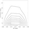Fig. 8 Isocontour plots of the joint distribution of the inclination of the stellar rotation axis vs. the absolute value of the difference between the spot rotation periods for ϵ Eridani.

5.3. DR in our sample of stars

For the eight stars in our sample, including the Sun, we determine the best intervals for measuring the DR according to the method introduced in Sect. 3.3 and illustrated by the case of Kepler-30 in Sect. 5.2.1. The beginning and the end of these intervals are indicated for each star in Table 2, together with the uniform priors applied to the model parameters. The origin of the time is in all cases the first observation of the corresponding time series (cf. Sect. 2), while the other symbols are defined in Sect. 3.2. The longitude intervals are defined as the maximum allowed deviations from the initial point of the MCMC chain that correspond to the parameters giving the minimum ${\mathit{\chi }}_{\mathrm{DR}}^{\mathrm{2}}$ (see below for details).

For the Sun, HD 52265, and HD 181906, the MCMC chains do not properly converge as indicated by values of the parameter R > 1.2 for one or several of the model parameters (see Table 3). No significant improvement is obtained by applying the recipes described in Sect. 3.5 or by reducing the acceptance threshold for the chi square variation to values as low as 0.1−0.5 percent. For these stars, with the exception of the Sun, we repeat the analyses with a different interval to confirm that the result does not depend on the particular interval (cf. Table 2). The values of R given in Table 3 provide some information on the model parameter chains that have not reached a proper convergence or mixing. We note that R is undefined when the corresponding model parameter has been fixed in an attempt to improve the convergence as in the case of the Sun (cf. Sect. 3.2 in Verde et al. 2003). Values of R lower than the acceptable threshold of 1.2 for only a subset of the model parameters do not imply that the marginal distributions of the corresponding parameters have converged, because the correlations with the parameters having R > 1.2 make them unreliable. Therefore, we require that R < 1.2 for all the parameters in order to use the a posteriori distributions derived with the MCMC approach for the individual parameters. It is interesting to note that all these stars for which MCMCs do not convergence are characterized by an autocorrelation function with secondary peaks that decrease rapidly with increasing time lag, thereby indicating a fast spot evolution. Previous analysis based on Lomb-scargle periodogram and multi-spot models have provided some evidence of DR in those stars, although they also detected a rapid intrinsic spot evolution that could affect the determination, possibly mimicking a DR signal (Ballot et al. 2011; Mosser et al. 2009).

For CoRoT-6, KIC 7765135, KIC 7985370, KIC 8429280, and Kepler-30, we are able to compute convergent and well-mixed MCMCs by applying the recipes in Sect. 3.5 and fixing the threshold for the chi square acceptance between one and five percent above the minimum (cf. Table 3). For Kepler-30 and KIC 7765135, we find maximum values of R of 1.197 and 1.067 considering chains of 36 and 500 million steps, respectively. In the case of CoRoT-6, the maximum value of R is 1.186 considering a chain of 128 million steps. For KIC 7985370, it has been necessary to fix the inclination of the rotation axis and the colatitudes of the starspots at the values corresponding to the minimum of the chi square to obtain a maximum R equal to 1.125 for a chain of 180 million steps. Therefore, the R values corresponding to those fixed parameters are undefined. For KIC 8429280, we find strong correlations among the reference flux F₀, the inclination i, and the spot area a₂ that can be treated with the approach described in Sect. 3.5, which yields a maximum R of 1.010 after computing a chain of 36 million steps. As a consequence of the correlations explicitly included in the model, the values of R corresponding to those parameters are the same in Table 3.

Fig. 9 A posteriori distributions of the rotation periods of the two spots as derived from MCMC analysis for CoRoT-6. The solid line refers to the distribution of the rotation period of the first spot, the dashed line to that of the second.

Fig. 10 Same as Fig. 9 for KIC 7765135.

Fig. 11 Same as Fig. 9 for KIC 7985370.

Fig. 12 Same as Fig. 9 for the distributions of the rotation periods of the two spots of KIC 8429280.

Fig. 13 Same as Fig. 9 for Kepler-30.

In Table 4, we list the rotation periods of the two starspots with their standard deviations as derived from the a posteriori marginal distributions of P₁ and P₂ as well as the corresponding relative amplitude of the differential rotation ΔP/P with its standard deviation for our sample stars. The distributions of the rotation periods of the two starspots are plotted in Figs. 9 (CoRoT-6), 10 (KIC 7765135), 11 (KIC 7985370), 12 (KIC 8429280), and 13 (Kepler-30). The area of the intersection between the distributions is virtually zero, thus providing evidence for DR in the framework of our model.

The amplitude of the DR determined by our method depends of course on the specific interval considered because spots can appear at different latitudes in late-type stars. The latitude range is wider in more active stars than in the Sun (see, e.g., Moss et al. 2011), thus making the differences larger for CoRoT-6 and the young Sun-like stars in our sample. Specifically, from the modelling of another interval for CoRoT-6, we find ΔP/P = 0.259 ± 0.003, while for, say, KIC 8429280, another interval gives ΔP/P = 0.011 ± 3.73 × 10^-5, where the standard deviations are derived from the a posteriori distributions given by the MCMC method. This should be kept in mind when comparing the present results with previous ones. For CoRoT-6, Lanza et al. (2011) find ΔP/P of about half the present value by tracing the migration of the active longitudes, not of the individual spots. A remarkable difference in those migration rates has indeed been found in CoRoT-2 that could explain the present result (cf. Lanza et al. 2009a). Our spot rotation periods fall within the range found by Frasca et al. (2011) for KIC 8429280, while they are close but slightly outside the ranges found for KIC 7765135 and KIC 7985370 by Fröhlich et al. (2012). However, those models use seven to nine evolving spots to fit the whole time series instead of two fixed spots applied to fit a data interval.

6. Conclusions

We have introduced a method of searching for differential rotation (DR) signals in high-precision photometric time series of the late-type stars acquired by space-borne telescopes (see Sect. 3). The even sampling of the time series allowed us to apply an autocorrelation to measure the timescale of the intrinsic evolution of the spot pattern that limits the possibility of measuring DR. We selected a sample of eight stars for which previous determinations of DR based on photometry were available along with some information on the inclination of the stellar rotation axis. We added the Sun as a star to this sample to study the rotation of solar analogues. We found that a significant DR can be detected when the relative height of the second maximum in the autocorrelation function is at least 0.6−0.7. In this case, we subdivided the time series into intervals the duration of which was shorter than the typical timescale of starspot evolution, although long enough to reveal the drift of the spot longitudes produced by DR. The best interval was then selected by comparing the best fits obtained with a simple two-spot model with and without DR. For that interval, a fully Bayesian analysis was undertaken by means of an MCMC approach to assess the significance of DR and determine its most probable value and uncertainty.

We found that the amplitude of the DR derived with our method is generally consistent with previous results when the different assumptions of the other approaches are considered. The advantage of our approach is the simplicity of the spot model that allows us to run MCMCs with tens or hundreds of million steps to study the a posteriori distribution of the parameters. This is particularly useful in spot modelling given the strong correlations among different parameters. We took advantage of the available information on the inclination of the stellar rotation axis to fix the a priori distribution of the inclination that is strongly correlated with the colatitudes and the unprojected areas of starspots in our model. Other correlations may become important when the signal-to-noise ratio of the photometry is low, spots are rapidly evolving (τ_s ≲ (2.5−3.0)P), or the DR relative amplitude is small (ΔP/P ≲ 0.01). They severely hamper the proper mixing and convergence of the MCMC procedure, although their effect can be controlled as described in Sect. 3.5, provided that a clear signal of DR is present in the light curve.

In the case of stars more active than the Sun, we find that the measured amplitude of DR depends on the specific time interval considered. In general, our approach only provides a lower limit to the amplitude of surface DR. We did not attempt to extract the amplitude and sign of the pole-equator shear as in other works (e.g., Fröhlich et al. 2012) because spot colatitude and inclination of the stellar spin axis are highly correlated in our simple spot model. On the other hand, an independent estimate of the inclination is generally not available, except in the case of close eclipsing binaries or transiting star-planet systems.

Acknowledgments

The authors are grateful to an anonymous referee for a careful reading of the manuscript and valuable comments that helped to improve their work. AFL is grateful to Drs. A. S. Bonomo, H.-E. Fröhlich, D. Gandolfi, and Prof. S. Ingrassia for useful discussions. MLC acknowledges the CAPES Brazilian agency for a PDSE fellowship (BEX-9103/12-0) and I. C. Leao for providing software for light curve treatment. Research activities of the Stellar Board of the Federal University of Rio Grande do Norte are supported by CNPq and FAPERN Brazilian agencies. J.R.M. and M.L.C. also acknowledges the INCT INEspaço. This investigation made use of data from MOST (a Canadian Space Agency mission, jointly operated by Microsatellite Systems Canada Inc. (MSCI; formerly Dynacon Inc.), the University of Toronto Institute for Aerospace Studies, and the University of British Columbia, with the assistance of the University of Vienna), CoRoT (a space mission developed and operated by the CNES, with participation of the Science Programmes of ESA, ESA’s RSSD, Austria, Belgium, Brazil, Germany, and Spain), and Kepler (a NASA space mission), the public availability of which is gratefully acknowledged.

References

Appendix A: Correlations between parameters adopted in MCMC spot modelling

To justify the correlations among parameters adopted in some of our MCMC modelling, we consider that they are most evident when a given spot j produces its maximum photometric effect, that is when μ as given by Eq. (10) is at its maximum ${\mathit{\mu }}_{\mathit{j}}^{\mathrm{\left(}\mathrm{m}\mathrm{\right)}}$. This occurs at an epoch ${\mathit{t}}_{\mathit{j}}^{\mathrm{\left(}\mathrm{m}\mathrm{\right)}}$ when the phase ${\mathit{\lambda }}_{\mathit{j}}\mathrm{+}{\mathrm{\Omega }}_{\mathit{j}}\mathrm{(}{\mathit{t}}_{\mathit{j}}^{\mathrm{\left(}\mathrm{m}\mathrm{\right)}}\mathrm{-}{\mathit{t}}_{\mathrm{0}}\mathrm{)}\mathrm{=}\mathrm{0}$, that is ${\mathit{t}}_{\mathit{j}}^{\mathrm{\left(}\mathrm{m}\mathrm{\right)}}\mathrm{-}{\mathit{t}}_{\mathrm{0}}\mathrm{=}\mathrm{-}{\mathit{\lambda }}_{\mathit{j}}\mathit{/}{\mathrm{\Omega }}_{\mathit{j}}$. At that epoch we have: ${\mathit{\mu }}_{\mathit{j}}^{\mathrm{\left(}\mathrm{m}\mathrm{\right)}}\mathrm{=}\cos \mathrm{(}\mathit{i}\mathrm{-}{\mathit{\theta }}_{\mathit{j}}\mathrm{)}\mathit{.}$(A.1)From Eqs. (A.1) and (9), we see that the maximum photometric effect of a given spot is not changed when δθ_j = δi, thus establishing a strong correlation between the variations of its colatitude and of the inclination of the stellar rotation axis.

Another correlation comes from the phase of maximum spot visibility that after variation yields: $\mathit{\delta }{\mathit{\lambda }}_{\mathit{j}}\mathrm{+}\mathit{\delta }{\mathrm{\Omega }}_{\mathit{j}}\mathrm{(}{\mathit{t}}_{\mathit{j}}^{\mathrm{\left(}\mathrm{m}\mathrm{\right)}}\mathrm{-}{\mathit{t}}_{\mathrm{0}}\mathrm{)}\mathrm{=}\mathrm{0}\mathit{,}$(A.2)where ${\mathit{t}}_{\mathit{j}}^{\mathrm{\left(}\mathrm{m}\mathrm{\right)}}\mathrm{-}{\mathit{t}}_{\mathrm{0}}$ is not varied because the epoch of maximum visibility is constrained by a relative minimum in the flux along the observed time series. Since ${\mathit{t}}_{\mathit{j}}^{\mathrm{\left(}\mathrm{m}\mathrm{\right)}}\mathrm{-}{\mathit{t}}_{\mathrm{0}}\mathrm{=}\mathrm{-}{\mathit{\lambda }}_{\mathit{j}}\mathit{/}{\mathrm{\Omega }}_{\mathit{j}}$ and δΩ_j/Ω_j = −δP_j/P_j, we obtain the correlation: $\mathit{\delta }{\mathit{\lambda }}_{\mathit{j}}\mathit{/}{\mathit{\lambda }}_{\mathit{j}}\mathrm{=}\mathrm{-}\mathit{\delta }{\mathit{P}}_{\mathit{j}}\mathit{/}\mathit{P}j$(A.3)between the longitude λ_j and the rotation period P_j of a given spot.

All Tables

All Figures

	Fig. 1 Photometric time series of the Sun and the other considered stars. The flux has been normalized to the maximum value observed along each time series.
In the text

	Fig. 2 Autocorrelation functions of the light curves of the stars considered in our sample. The dotted lines indicate the ± σ interval (see the text).
In the text

	Fig. 3 Autocorrelation function of the light curve of KIC 8429280 extended up to τ/Prot = 60 to show the beatings of the amplitude. The dotted lines indicate the ± σ interval (see the text).
In the text

	Fig. 4 Distribution of the residuals of the composite best fit to the entire time series of Kepler-30 obtained with the two-spot model with DR for M = 51. The dashed line is a Gaussian best fit to the distribution.
In the text

	Fig. 5 The optical flux of ϵ Eridani (filled dots) vs. the time, together with the best fits obtained with our two-spot model with DR (solid line) or rigid rotation (dashed line).
In the text

Fig. 6 Frequency marginal distributions of the parameters of the two-spot model with DR for ϵ Eridani. From top to bottom: area of the first (solid line) and the second (dashed line) spot; colatitude of the first (solid line) and the second (dashed line) spot; deviation of the longitude of the first spot (solid line) and of the second spot (dashed line) from their initial longitudes, respectively; rotation period of the first spot (solid line) and of the second spot (dashed line); reference flux; inclination of the stellar spin axis.

In the text

	Fig. 7 Isocontour plots of the joint distribution of the inclination of the stellar rotation axis vs. the colatitude of the first spot for ϵ Eridani.
In the text

	Fig. 8 Isocontour plots of the joint distribution of the inclination of the stellar rotation axis vs. the absolute value of the difference between the spot rotation periods for ϵ Eridani.
In the text

	Fig. 9 A posteriori distributions of the rotation periods of the two spots as derived from MCMC analysis for CoRoT-6. The solid line refers to the distribution of the rotation period of the first spot, the dashed line to that of the second.
In the text

	Fig. 10 Same as Fig. 9 for KIC 7765135.
In the text

	Fig. 11 Same as Fig. 9 for KIC 7985370.
In the text

	Fig. 12 Same as Fig. 9 for the distributions of the rotation periods of the two spots of KIC 8429280.
In the text

	Fig. 13 Same as Fig. 9 for Kepler-30.
In the text

References

- Ammler-von Eiff, M., & Reiners, A. 2012, A&A, 542, A116 [NASA ADS] [CrossRef] [EDP Sciences] [Google Scholar]
- Anderson, O. 1976, Time series analysis and forecasting: the Box-Jenkins approach (London: Butterworths) [Google Scholar]
- Auvergne, M., Bodin, P., Boisnard, L., et al. 2009, A&A, 506, 411 [NASA ADS] [CrossRef] [EDP Sciences] [Google Scholar]
- Ballot, J., Gizon, L., Samadi, R., et al. 2011, A&A, 530, A97 [NASA ADS] [CrossRef] [EDP Sciences] [Google Scholar]
- Balona, L. A. 2013, MNRAS, 431, 2240 [NASA ADS] [CrossRef] [Google Scholar]
- Barnes, J. R., Collier Cameron, A., Lister, T. A., Pointer, G. R., & Still, M. D. 2005, MNRAS, 356, 150 [Google Scholar]
- Basri, G., Walkowicz, L. M., Batalha, N., et al. 2011, AJ, 141, 20 [NASA ADS] [CrossRef] [Google Scholar]
- Berdyugina, S. V., & Henry, G. W. 2007, ApJ, 659, L157 [NASA ADS] [CrossRef] [Google Scholar]
- Borucki, W. J., Koch, D., Basri, G., et al. 2010, Science, 327, 977 [NASA ADS] [CrossRef] [PubMed] [Google Scholar]
- Brandenburg, A., & Subramanian, K. 2005, Phys. Rep., 417, 1 [NASA ADS] [CrossRef] [Google Scholar]
- Bumba, V. 1963, Bull. Astron. Inst. Czechosl., 14, 91 [Google Scholar]
- Butler, R. P., Vogt, S. S., Marcy, G. W., et al. 2000, ApJ, 545, 504 [NASA ADS] [CrossRef] [Google Scholar]
- Claret, A., & Bloemen, S. 2011, A&A, 529, A75 [NASA ADS] [CrossRef] [EDP Sciences] [Google Scholar]
- Cowan, N. B., Fuentes, P. A., & Haggard, H. M. 2013, MNRAS, 434, 2465 [NASA ADS] [CrossRef] [Google Scholar]
- Croll, B. 2006, PASP, 118, 1351 [NASA ADS] [CrossRef] [Google Scholar]
- Croll, B., Walker, G. A. H., Kuschnig, R., et al. 2006, ApJ, 648, 607 [NASA ADS] [CrossRef] [Google Scholar]
- Deheuvels, S., García, R. A., Chaplin, W. J., et al. 2012, ApJ, 756, 19 [NASA ADS] [CrossRef] [Google Scholar]
- De Medeiros, J. R., Ferreira Lopes, C. E., Leão, I. C., et al. 2013, A&A, 555, A63 [NASA ADS] [CrossRef] [EDP Sciences] [Google Scholar]
- Dikpati, M., & Charbonneau, P. 1999, ApJ, 518, 508 [NASA ADS] [CrossRef] [Google Scholar]
- Donahue, R. A., & Keil, S. L. 1995, Sol. Phys., 159, 53 [NASA ADS] [CrossRef] [Google Scholar]
- Donahue, R. A., Saar, S. H., & Baliunas, S. L. 1996, ApJ, 466, 384 [NASA ADS] [CrossRef] [Google Scholar]
- Donahue, R. A., Dobson, A. K., & Baliunas, S. L. 1997a, Sol. Phys., 171, 191 [NASA ADS] [CrossRef] [Google Scholar]
- Donahue, R. A., Dobson, A. K., & Baliunas, S. L. 1997b, Sol. Phys., 171, 211 [NASA ADS] [CrossRef] [Google Scholar]
- Donati, J.-F., & Collier Cameron, A. 1997, MNRAS, 291, 1 [NASA ADS] [CrossRef] [Google Scholar]
- Donati, J.-F., Semel, M., Carter, B. D., Rees, D. E., & CollierCameron, A. 1997, MNRAS, 291, 658 [NASA ADS] [CrossRef] [MathSciNet] [Google Scholar]
- Edelson, R. A., & Krolik, J. H. 1988, ApJ, 333, 646 [NASA ADS] [CrossRef] [Google Scholar]
- Epstein, C. R., & Pinsonneault, M. H. 2014, ApJ, 780, 159 [NASA ADS] [CrossRef] [Google Scholar]
- Fabrycky, D. C., Ford, E. B., Steffen, J. H., et al. 2012, ApJ, 750, 114 [NASA ADS] [CrossRef] [Google Scholar]
- Fligge, M., Solanki, S. K., & Unruh, Y. C. 2000, A&A, 353, 380 [NASA ADS] [Google Scholar]
- Ford, E. B. 2006, ApJ, 642, 505 [NASA ADS] [CrossRef] [Google Scholar]
- Frasca, A., Fröhlich, H.-E., Bonanno, A., et al. 2011, A&A, 532, A81 [NASA ADS] [CrossRef] [EDP Sciences] [Google Scholar]
- Fröhlich, C., Romero, J., Roth, H., et al. 1995, Sol. Phys., 162, 101 [NASA ADS] [CrossRef] [Google Scholar]
- Fröhlich, C., Andersen, B. N., Appourchaux, T., et al. 1997a, Sol. Phys., 170, 1 [NASA ADS] [CrossRef] [Google Scholar]
- Fröhlich, C., Crommelynck, D. A., Wehrli, C., et al. 1997b, Sol. Phys., 175, 267 [NASA ADS] [CrossRef] [Google Scholar]
- Fröhlich, H.-E. 2007, Astron. Nachr., 328, 1037 [NASA ADS] [CrossRef] [Google Scholar]
- Fröhlich, H.-E., Frasca, A., Catanzaro, G., et al. 2012, A&A, 543, A146 [NASA ADS] [CrossRef] [EDP Sciences] [Google Scholar]
- García, R. A., Régulo, C., Samadi, R., et al. 2009, A&A, 506, 41 [NASA ADS] [CrossRef] [EDP Sciences] [Google Scholar]
- Gondoin, P. 2008, A&A, 478, 883 [NASA ADS] [CrossRef] [EDP Sciences] [Google Scholar]
- Goupil, M. J., Mosser, B., Marques, J. P., et al. 2013, A&A, 549, A75 [NASA ADS] [CrossRef] [EDP Sciences] [Google Scholar]
- Hempelmann, A., & Donahue, R. A. 1997, A&A, 322, 835 [NASA ADS] [Google Scholar]
- Howe, R. 2009, Liv. Rev. Sol. Phys., 6, 1 [Google Scholar]
- Howe, R., Christensen-Dalsgaard, J., Hill, F., et al. 2000, Science, 287, 2456 [NASA ADS] [CrossRef] [PubMed] [Google Scholar]
- Knobloch, E., & Spruit, H. C. 1982, A&A, 113, 261 [NASA ADS] [Google Scholar]
- Kovári, Z., Bartus, J., Strassmeier, K. G., et al. 2007, A&A, 474, 165 [NASA ADS] [CrossRef] [EDP Sciences] [Google Scholar]
- Küker, M., Rüdiger, G. 2005, A&A, 433, 1023 [NASA ADS] [CrossRef] [EDP Sciences] [Google Scholar]
- Labonte, B. J. 1984, ApJ, 276, 335 [NASA ADS] [CrossRef] [Google Scholar]
- Lanza, A. F. 2007, A&A, 471, 1011 [NASA ADS] [CrossRef] [EDP Sciences] [Google Scholar]
- Lanza, A. F., Rodonò, M., & Zappalà, R. A. 1993, A&A, 269, 351 [NASA ADS] [Google Scholar]
- Lanza, A. F., Rodonò, M., & Zappalà, R. A. 1994, A&A, 290, 861 [NASA ADS] [Google Scholar]
- Lanza, A. F., Rodonò, M., Pagano, I., Barge, P., & Llebaria, A. 2003, A&A, 403, 1135 [NASA ADS] [CrossRef] [EDP Sciences] [Google Scholar]
- Lanza, A. F., Rodonò, M., & Pagano, I. 2004, A&A, 425, 707 [NASA ADS] [CrossRef] [EDP Sciences] [Google Scholar]
- Lanza, A. F., Piluso, N., Rodonò, M., Messina, S., & Cutispoto, G. 2006, A&A, 455, 595 [NASA ADS] [CrossRef] [EDP Sciences] [Google Scholar]
- Lanza, A. F., Bonomo, A. S., & Rodonò, M. 2007, A&A, 464, 741 [NASA ADS] [CrossRef] [EDP Sciences] [Google Scholar]
- Lanza, A. F., Pagano, I., Leto, G., et al. 2009a, A&A, 493, 193 [NASA ADS] [CrossRef] [EDP Sciences] [Google Scholar]
- Lanza, A. F., Aigrain, S., Messina, S., et al. 2009b, A&A, 506, 255 [NASA ADS] [CrossRef] [EDP Sciences] [Google Scholar]
- Lanza, A. F., Bonomo, A. S., Pagano, I., et al. 2011, A&A, 525, A14 [NASA ADS] [CrossRef] [EDP Sciences] [Google Scholar]
- Lehtinen, J., Jetsu, L., Hackman, T., Kajatkari, P., & Henry, G. W. 2011, A&A, 527, A136 [NASA ADS] [CrossRef] [EDP Sciences] [Google Scholar]
- Lehtinen, J., Jetsu, L., Hackman, T., Kajatkari, P., & Henry, G. W. 2012, A&A, 542, A38 [NASA ADS] [CrossRef] [EDP Sciences] [Google Scholar]
- Liddle, A. R. 2007, MNRAS, 377, L74 [NASA ADS] [Google Scholar]
- MacKay, D. J. C. 2003, Information Theory, Inference, Learning Algorithms (Cambridge: Cambridge Univ. Press), 30.1 [Google Scholar]
- Markwardt, C. B. 2009, Astronomical Data Analysis Software and Systems XVIII, ASP Conf. Ser., 411, 251 [NASA ADS] [Google Scholar]
- MartinezPillet, V., Moreno-Insertis, F., & Vazquez, M. 1993, A&A, 274, 521 [NASA ADS] [Google Scholar]
- Mathis, S., Le Poncin-Lafitte, C., & Remus, F. 2012, Lect. Notes Phys., 861 (Berlin: Springer Verlag), 255 [Google Scholar]
- McQuillan, A., Aigrain, S., & Mazeh, T. 2013, MNRAS, 432, 1203 [NASA ADS] [CrossRef] [MathSciNet] [Google Scholar]
- Messina, S., & Guinan, E. F. 2002, A&A, 393, 225 [Google Scholar]
- Messina, S., & Guinan, E. F. 2003, A&A, 409, 1017 [NASA ADS] [CrossRef] [EDP Sciences] [Google Scholar]
- Moss, D., Sokoloff, D., & Lanza, A. F. 2011, A&A, 531, A43 [NASA ADS] [CrossRef] [EDP Sciences] [Google Scholar]
- Mosser, B., Baudin, F., Lanza, A. F., et al. 2009, A&A, 506, 245 [NASA ADS] [CrossRef] [EDP Sciences] [Google Scholar]
- Mosser, B., Goupil, M. J., Belkacem, K., et al. 2012, A&A, 548, A10 [NASA ADS] [CrossRef] [EDP Sciences] [Google Scholar]
- Neal, R. M. 1993, Probabilistic inference using Markov Chain Monte Carlo methods, Tech. Rep. CRG-TR-93-1 (Dept. of Computer Science, Univ. of Toronto) [Google Scholar]
- Press, W. H., Teukolsky, S. A., Vetterling, W. T., & Flannery, B. P. 2002, Numerical recipes in C++: the art of scientific computing, Chap. 15 (Cambridge: Cambridge Univ. Press) [Google Scholar]
- Reiners, A. 2006, A&A, 446, 267 [NASA ADS] [CrossRef] [EDP Sciences] [Google Scholar]
- Reiners, A., & Schmitt, J. H. M. M. 2003, A&A, 398, 647 [NASA ADS] [CrossRef] [EDP Sciences] [Google Scholar]
- Reinhold, T., & Reiners, A. 2013, A&A, 557, A11 [NASA ADS] [CrossRef] [EDP Sciences] [Google Scholar]
- Reinhold, T., Reiners, A., & Basri, G. 2013, A&A, 560, A4 [NASA ADS] [CrossRef] [EDP Sciences] [Google Scholar]
- Rucinski, S., Carroll, K., Kuschnig, R., Matthews, J., & Stibrany, P. 2003, Adv. Space Res., 31, 371 [NASA ADS] [CrossRef] [Google Scholar]
- Rüdiger, G. 1989, Differential rotation and stellar convection (New York: Gordon & Breach Science Publ.) [Google Scholar]
- Russell, H. N. 1906, ApJ, 24, 1 [NASA ADS] [CrossRef] [Google Scholar]
- Sanchis-Ojeda, R., Fabrycky, D. C., Winn, J. N., et al. 2012, Nature, 487, 449 [NASA ADS] [CrossRef] [PubMed] [Google Scholar]
- Scharlemann, E. T. 1981, ApJ, 246, 292 [NASA ADS] [CrossRef] [Google Scholar]
- Scharlemann, E. T. 1982, ApJ, 253, 298 [NASA ADS] [CrossRef] [Google Scholar]
- Silva-Valio, A., & Lanza, A. F. 2011, A&A, 529, A36 [NASA ADS] [CrossRef] [EDP Sciences] [Google Scholar]
- Smirnov, V. I. 1964, in A course of higher mathematics, Vol. II (Oxford: Pergamon Press), 157 [Google Scholar]
- Strassmeier, K. G. 2009, A&ARv, 17, 251 [NASA ADS] [CrossRef] [Google Scholar]
- Twicken, J. D., Chandrasekaran, H., Jenkins, J. M., et al. 2010, Proc. SPIE, 7740, 77401U [NASA ADS] [CrossRef] [Google Scholar]
- Walker, G., Matthews, J., Kuschnig, R., et al. 2003, PASP, 115, 1023 [NASA ADS] [CrossRef] [Google Scholar]
- Verde, L., Peiris, H. V., Spergel, D. N., et al. 2003, ApJS, 148, 195 [NASA ADS] [CrossRef] [Google Scholar]