| Issue |
A&A
Volume 549, January 2013
|
|
|---|---|---|
| Article Number | A107 | |
| Number of page(s) | 9 | |
| Section | Interstellar and circumstellar matter | |
| DOI | https://doi.org/10.1051/0004-6361/201220362 | |
| Published online | 07 January 2013 | |
Two radio supernova remnants discovered in the outer Galaxy
1
Department of Physics & AstronomyBrandon University 270-18th
Street,
Brandon,
MB
R7A 6A9,
Canada
e-mail: This email address is being protected from spambots. You need JavaScript enabled to view it.
2
National Research Council of Canada, Emerging Technologies –
National Science Infrastructure, Dominion Radio Astrophysical
Observatory, PO Box
248, Penticton BC,
V2A 6J9,
Canada
3
Dept. of Physics & Astronomy, University of British
Columbia Okanagan, 3333 University Way, Kelowna BC
V1V 1V7,
Canada
4
Max-Planck-Institut für Radioastronomie,
Auf dem Hügel 69, 53121
Bonn,
Germany
5
Dept. of Physics & Astronomy, University of Calgary, 2500
University Drive NW Calgary, AB
T2N 1N4,
Canada
6
Dept. of Physics & Astronomy University of
Manitoba, Winnipeg,
MB
R3T 2N2,
Canada
Received: 10 September 2012
Accepted: 16 November 2012
Abstract
Context. New and existing large-scale radio surveys of the Milky Way at centimetre wavelengths can play an important role in uncovering the hundreds of expected but missing supernova remnants in the Galaxy’s interstellar medium. We report on the discovery of two supernova remnants (SNRs) designated G152.4−2.1 and G190.9−2.2, using Canadian Galactic Plane Survey data.
Aims. The aims of this paper are, first, to present evidence that favours the classification of both sources as SNRs, and, second, to describe basic parameters (integrated flux density, spectrum, and polarization) as well as properties (morphology, line-of-sight velocity, distance and physical size) to facilitate and motivate future observations.
Methods. Spectral and polarization parameters are derived from multiwavelength data from existing radio surveys carried out at wavelengths between 6 and 92 cm. In particular for the source G152.4−2.1 we also use new observations at 11 cm done with the Effelsberg 100 m telescope. The interstellar medium around the discovered sources is analyzed using 1-arcmin line data from neutral hydrogen (H i) and 45-arcsec 12CO(J = 1 → 0).
Results. G152.4−2.1 is a barrel shaped SNR with two opposed radio-bright polarized flanks on the north and south. The remnant, which is elongated along the Galactic plane is evolving in a more-or-less uniform medium. G190.9−2.2 is also a shell-type remnant with east and west halves elongated perpendicular to the plane, and is evolving within a low-density region bounded by dense neutral hydrogen in the north and south, and molecular (12CO) clouds in the east and west. The integrated radio continuum spectral indices are −0.65 ± 0.05 and −0.66 ± 0.05 for G152.4−2.1 and G190.9−2.2 respectively. Both SNRs are approximately 1 kpc distant, with G152.4−2.1 being larger (32 × 30 pc in diameter) than G190.9−2.2 (18 × 16 pc). These two remnants are the lowest surface brightness SNRs yet catalogued at Σ1 GHz ≲ 5 × 10-23 W m-2 Hz-1 sr-1.
Key words: ISM: supernova remnants / ISM: general
© ESO, 2013
1. Introduction
Supernovae are the predominant source of new energy and elememtal input into the interstellar medium (ISM). Shock waves from supernova blasts carve out hot ionized tunnels in the ISM, sweep up and ionize the gas in the neutral ISM, twist and contort the Galactic magnetic field, compress nearby interstellar clouds and could also trigger star formation and create the soup of cosmic rays in the Galactic environment that plays an important role in pressure balance in the Milky Way ISM and star formation (among other things). Besides the detailed understanding of individual physical properties of supernova remnants (SNRs) that is needed to get a more global picture of their place in the ISM, a simple accurate count of the number of Galactic SNRs is required. Assuming a mean age of radio shell-type SNRs of ≳60 000 yrs (Frail et al. 1994) and a rate of one SNe per 30−50 years in spiral galaxies like the Milky Way (Koo et al. 2006), the ISM should play host to between one and two-thousand radio supernova remnants at any given epoch. However in 2009 only 274 SNRs were catalogued in the Milky Way (Green 2009), and although this has increased to ≥ 310 today in light of recent observations (see catalogue1 of Ferrand & Safi-Harb 2012) there are still many “missing” SNRs, undoubtedly due to difficulties in identifying very faint objects. The “missing SNRs problem” is also apparent in models of the angular distribution of H ii regions and SNRs in the Galaxy which predict about 1000 Galactic SNRs (Li et al. 1991).
Many radio-emitting SNRs descend from type Ib, Ic and II (core collapse) supernova events, and are more likely to be evolving in a low density environment created by the stellar wind(s) of their massive and powerful progenitor (and cluster companions). The majority of Galactic SNRs in the catalogue of Kothes et al. (2006) are found in the adiabatic expansion phase, where energy from their shocks is being efficiently converted into radio, X-ray and/or optical radiation. This indicates an observational bias favouring SNRs that are significantly interacting with their local ISM environment, and suggests that many SNRs, whose shocks are still more-or-less freely expanding inside pre-made cavities and have not encountered the inner walls of the bubbles created by stellar winds, remain unobserved. Discoveries of new SNRs within high-sensitivity, high-resolution and wide-field radio continuum and polarimetric surveys of the Galactic plane (for example Brogan et al. 2006; Gao et al. 2011) are becoming common now that such surveys are more widely available. This success at alleviating the missing SNRs problem is being used to motivate a new generation of surveys (e.g. GALFACTS, POSSUM, LOFAR, and surveys to be performed by the SKA). Their sensitivity to all angular structures and their wide fields allows detection and study of large, low-surface brightness objects in the context of their local Galactic background, while their high-resolution lowers the confusion limit, allowing one to distinguish small angular structures from large ones (and to separate them). The Canadian Galactic Plane Survey (CGPS, Taylor et al. 2003) is the original such survey, and probes the ionized, neutral, and magneto-ionic ISM over unprecedented spatial dynamic range. Since 2001 this dataset has enabled the discovery of 7 new SNRs in the 1st and 2nd quadrants of longitude (Kothes et al. 2001; Kothes 2003; Kothes et al. 2005; Tian et al. 2007; Kerton et al. 2007), and allowed new insights into the SNR population in our Galaxy. In this paper we add two of the faintest-known SNRs to the list of catalogued remnants in our Galaxy.
The new SNR candidates in this paper were discovered in two individual CGPS 21 cm mosaics that had been source-subtracted and subsequently smoothed to gain S/N and better reveal large unseen extended emission in the survey. The two low surface-brightness shell-type SNRs are designated G152.4−2.1 and G190.9−2.2 (names from Galactic ℓ,b coordinates of their geometric centres). Flux densities at five radio wavelengths (λ6 cm, 11, 21, 74 and 92 cm; in frequency ν = 4.8 GHz, 2.7 GHz, 1420 MHz, 408 MHz and 327 MHz respectively) are measured with Stokes I data. Polarized intensity maps with B-field vectors from Stokes Q and U maps are presented at λ6, 11, and 21 cm (for G190.9−2.2 only 6 cm and 21 cm polarization data are available). Steep integrated radio spectra for each of the respective 1 5 and 1° diameter shells of G152.4−2.1 and G190.9−2.2 show the predominantly non-thermal nature of the sources. Finally we present 1-arcminute resolution H i and 12CO(J = 1 → 0) line channel maps towards each remnant and estimate LSR velocities, kinematic distances and physical diameters for each.
The primary purpose of this paper is to announce the discovery of the objects, present evidence for their identification as SNRs and provide only the basic measurements that can be reliably gleaned from survey data. It is hoped this will aid future specialized observations of both objects, observations with deeper sensitivities which will be needed to embark on detailed studies of their physics (e.g. spatial and frequency variation of spectral indexes, relative amount of free-free thermal and sychrotron emission, age and shock velocities, etc.), beyond the scope of this discovery paper.
2. Observations
2.1. 21 cm and 74 cm
The 21 cm Stokes I,Q,U continuum and H i line, and 74 cm continuum data come from the CGPS, which is described in detail by Taylor et al. (2003). The release of the CGPS 21 cm Q and U maps are described by Landecker et al. (2010). For our purpose (a qualitative look at the polarization structure of the objects) we use the interferometer-only Q and U data without the large-scale structures restored. CGPS data were observed with the 7-antenna Synthesis Telescope (ST) of the Dominion Radio Astrophysical Observatory (DRAO). Near G152.4−2.1 the elliptical synthesized beam of this interferometer in the continuum is  at 21 cm, and
  at 74 cm. Near G190.9−2.2 these values become highly elliptical at
  and
and  . The practice of observing all baselines from 617 m to 12.9 m over 144 h per field leads to good sensitivity despite the relatively small 9-m diameter of the primary antennae: in the vicinity of G152.4−2.1 (G190.9−2.2) measured 1-sigma sensitivities are ΔTB = 60 mK (40 mK) in the 21 cm continuum, and 0.8 K (0.4 K) at 74 cm. In 21 cm Stokes Q they are ~100 mK (42 mK) and in Stokes U are 80 mK (41 mK). The more elongated synthesized beam near ℓ = 190° accounts for its lower noise. Emission from structures larger than those the shortest baseline of the ST can sample are added in from surveys by the Effelsberg 100 m, the Stockert 25 m and the DRAO 26 m telescopes. Data from single-dishes like these are of particular importance to restoring the true flux density of faint extended objects like new SNRs, which is missed by the incomplete spatial frequency sampling of ST images. The CGPS data used here are two of 84 mosaics designated “MST1” and “MEQ1”, which are all available to the community through the Canadian Astronomy Data Centre (CADC2).
2.2. 11 cm
11 cm data of the two new SNRs were obtained with the Effelsberg 100-m telescope. For G152.4−2.1 new observations were made between August 2006 and January 2007 with a two channel cooled receiver with a bandwidth of 80 MHz centered at 2639 MHz. The two circularly polarized 80 MHz wide channels were correlated by an Intermediate Frequency polarimeter, which records Stokes I, Q and U simultaneously. In addition, the 80 MHz bandwidth was split into 8 × 10 MHz wide channels to eliminate narrow-band interference and to measure possible large rotation measure (RM) variations. 3C 286 served as the main calibrator with a flux density of 10.4 Jy, 9.9% of linear polarization at a polarization angle of 33°. We observed a  large field centred on G152.4−2.1 by moving the telescope beam either along Galactic longitude or along Galactic latitude direction with a speed of 3′/s. The individual scans of each map have 2′ separation providing full sampling of the 4
 4 beam of the Effelsberg telescope at 2639 MHz. The standard data reduction software package, based on the NOD2 format (Haslam 1974) was used for the Effelsberg continuum observations. The maps in NOD2-format were edited for interference, and “scanning effects” were suppressed by applying the unsharp masking method (Sofue & Reich 1979). We ended up with nearly 15 coverages which were combined into the final map by using the weaving method described by Emerson & Graeve (1988). The rms-noise of the final maps was measured to be 2.5 mK (~1 mJy) for Stokes I and 1.5 mK for Stokes Q and U. Analysis of the narrow channel polarization data does not indicate the existence of large RM features exceeding 100 rad m-2 or more. Earlier low resolution RM data by Spoelstra (1984) indicate RMs around 0 rad/m2 in this direction of sky. By defining the pixels at the end of each scan to be zero, large-scale emission exceeding the size of the map may be lost, which is not an issue for studying a discrete continuum source within a field, but might affect Stokes Q and U.
For G190.9−2.2 we extracted total intensity data from the Effelsberg 11 cm (2695 MHz) Galactic plane survey3 described in Fürst et al. (1990), which has a sensitivity of about ΔTB = 16 mK. For details of the receiver used for this survey and the antenna response of the Effelsberg 100-m telescope see Reich et al. (1984).
2.3. 6 cm
Data at λ6 cm (ν = 4.8 GHz) in Stokes I, Q and U are from the Sino-German polarization survey of the Galactic plane, made with the Urumqi 25 m telescope at Nanshan Station, China (Sun et al. 2007; Gao et al. 2010). Basic parameters of this survey are a resolution of 95, and a measured 1-sigma sensitivity in our data of ΔTB ~ 1.5 mK in I and ~0.5 mK in Q and U. We have used the original Urumqi polarization data without the absolute WMAP corrections. These data already include emission of several degrees in extent (much larger than our objects) and so are appropriate for polarization studies of all but the largest discrete objects.
2.4. 92 cm and other frequencies
Stokes I data for G152.4−2.1 were taken from the Westerbork Northern Sky Survey4 (WENSS, Rengelink et al. 1997) at 92 cm (325 MHz). As this survey only extends north of declination +28.5 degrees, data for G190.9−2.2 is unavailable. The measured 1-sigma flux density variation in these data is about 3.5 mJy/beam, or ΔTB ≃ 10 K with the synthesized beam of 54″ × 54″/sin (δ). Due to the restriction on short observing baselines for the Westerbork interferometer (about ~36 m, or 1.5 times an antenna diameter), the WENSS survey misses flux from structures greater than about 14 degrees in size. This will impact the 92 cm flux density derived for G152.4−2.1 only in a small way.
A faint extended source at the position of G190.9−2.2 was catalogued by Kassim (1988) at 30.9 MHz. He did not identify the object he catalogued as NEK 190.9−2.3 as a SNR. Nonetheless the orientation and size of emission contours in his maps are similar to G190.9−2.2, and it is likely these are one and the same object. The integrated flux density listed by Kassim for NEK 190.9−2.3 is S30.9 MHz = 13.6 Jy ± 20%.
Dust emission from the objects was searched for in IRAS 12, 25, 60 and 100 μm, and MSX 8 μm infrared survey data, but no emission spatially correlated to either source’s radio morphology was found at any of these infrared wavelengths. The combined Wisconsin H-Alpha Mapper (WHAM) and Virgina Tech Spectral line Survey (VTSS) map made by Finkbeiner (2003) was also searched for Hα emission from each object (angular resolution ~6′). We describe the discovery of emission corresponding with the radio appearance of G190.9−2.2 in Sect. 3.2.
3. Appearance, integrated flux densities and spectra
To better represent extended continuum emission, unresolved “point” sources were first removed from each map. For 21, 74 and 92 cm data, sources down to signal-to-noise (S/N) ~ 2σ were readily found by automated source finder “findsrc”, which examines an image using a matched “point-source” wavelet filter to enhance point-like sources and locate them in an image. Sources are modelled with two-dimensional elliptical Gaussians plus a base level using the program “fluxfit”. Both routines are part of the DRAO Export Software Package, a modular software package of general and telescope-specific programs for processing and analysis of images made by the DRAO Synthesis Telescope (Higgs et al. 1997). 6 and 11 cm maps had relatively fewer unresolved sources since their resolution is much poorer, so the brightest individual sources were identified using the original 1-arcminute 21 cm map overlaid as a guide, and these were modelled and subtracted with fluxfit. For brevity we do not list derived source fluxes and coordinates in this paper. To aid in identifying the shell and its edges the 21, 74 and 92 cm maps were next smoothed to 44 (the resolution of the 11 cm maps). Noise for these final smoothed maps are 25 mK, 0.4 K, and 1.6 K (at 21, 74 and 92 cm respectively) for G152.4−2.1, while the noise level for G190.9−2.2 is 15 mK and 0.4 K at 21 and 74 cm respectively. It is these source-removed and smoothed maps that are shown in Figs. 1 and 2. White 21 cm contours are overlaid on each map for comparison, also derived from the smoothed 44 resolution map.
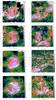 |
Fig. 1 Total (I) and polarized intensity (PI) contoured maps of G152.4−2.1. The emission features (colour bars in brightness temperature units of K, at right) are themselves outlined in thin black contours (levels indicated in the text above each panel). B-field vectors are overlaid on PI maps (length proportional to PI; scale differs between maps). Resolutions are 9 |
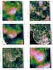 |
Fig. 2 Total (I) and polarized intensity (PI) contoured maps of G190.9−2.2. The emission features (colour bars in brightness temperature units of K, at right) are themselves outlined in thin black contours (levels indicated in the text above each panel). B-field vectors are overlaid on PI maps (length proportional to PI; scale differs between maps). Resolutions are 9 |
3.1. G152.4–2.1
We refer here to total intensity maps at λ6, 11, 21, 74, and 92 cm (4.8 GHz, 2.7 GHz, 1420 MHz, 408 MHz and 327 MHz) in Fig. 1. All total (I) and polarized intensity (PI) maps are presented in the colour-scheme of Green (2011). The emission structure of G152.4−2.1 is best seen in the 21 cm map. The very bright H ii region Sh2-206 is seen in the top-right corner of I maps (and 6 cm PI map). The radio emission from this SNR candidate consists of a pair of enhanced shells of emission with steep outer edges in the north and south. This is the typical “double loop” or “barrel”-shaped structure of a pure shell-type supernova remnant (see Manchester 1987; Gaensler 1998, for example), where two shells of enhanced radio emission are found atop a more diffuse central emission plateau which is likely generated by those parts of the source that are expanding towards us or moving away from us. Gaensler (1998) found that the orientation of these barrel-shaped SNRs is mostly parallel to the Galactic plane – as is the case for G152.4−2.1. He suggests that the reason for this shape is a combination of the uniform magnetic field structure which is preferentially parallel to the Galactic plane and the expansion into ISM structures which are elongated in longitudinal direction. Caswell (1977) also describes asymmetries in shell remnants as the outcome of ISM density gradients.
We determine the polarization properties of G152.4−2.1 using Stokes Q and U polarization maps at 6, 11, and 21 cm. In Fig. 1 we display polarized intensity images with B-vectors overlaid. The length of each vector is determined by the polarized intensity at that point; however, as the intention is simply to highlight the field’s direction, the scale in cm per mK is arbitrary from map to map in Figs. 1 and 2. Synchrotron emission from supernova remnants should be inherently polarized up to 70%; however Faraday rotation by the ISM and internal effects will depolarize this signal, and this depolarization is much more significant at 21 cm than at 6 cm, effectively scrambling low-frequency polarized intensity from a SNR. This effect can be easily seen in our polarized emission images. While there is a strong correlation between total power and polarization at 6 cm, the ambient polarization features become more and more dominant at longer wavelength.
G152.4−2.1 shows polarized intensity at 6 cm well correlated to continuum features, a good indicator that the emission is synchrotron in nature. The fractional polarization on the brightened regions of the shell is between 50 and 60%. G152.4−2.1 also seems to sit on an elongated slightly curved feature in polarized intensity more than 2 degrees in length. This large polarization filament seems to have a tangential intrinsic magnetic field as indicated by the B-vectors. At this high frequency, where effects of Faraday rotation should be small, the B-vectors of the SNR candidate indicate a tangential magnetic field in the northern shell, which is expected for a mature shell-type SNR. The southern shell shows a slight rotation of up to 30 degrees clockwise from a tangential structure, which requires a rotation measure of about −130 rad m-2. This would produce a rotation of about 90 degrees for polarization angles at 11 cm and we find the B-vectors in the 11 cm polarization image in this area to be almost radial. We did not produce a rotation measure map because at the lower frequencies the background/foreground polarization structures become more and more dominant and it is difficult to distinguish between them and genuine SNR emission.
From the polarized emission structure we conclude that the SNR is likely interacting with the large polarization filament, the nature of which is unclear. Its bright polarized emission implies an enhanced, compressed internal magnetic field. In this scenario the progenitor star of G152.4−2.1 would have exploded at the upper edge of this filament, sweeping up its magnetic field explaining the filament’s gap at the location of the SNR at 6 cm and the similarity of the B-vectors of both objects.
The 21 cm PI map is shown in Fig. 1. The only morphological correlation between the PI and I maps at 21 cm seems to be the distinct dark channel of depolarization that snakes west to east across most of the south shell’s face, which tightly follows the continuum around the southeast corner of G152.4−2.1. It is moderately consistent with a compressed magnetic field aligned in the east-west direction along the shell which cancels with the principally north-south field seen in the unrelated bright PI from the ISM immediately above it. Some of this bright PI emission on the shell’s western face at  ,
,  could originate with the SNR’s shell, but how much is impossible to say from these maps, as is its precise role in creating the depolarization “snake”.
3.2. G190.9–2.2
Total Power maps at 6, 11, 21 and 74 centimetres (4.8 GHz, 2.7 GHz, 1420 MHz, and 408 MHz) are shown in Fig. 2. The first impression of G190.9−2.2 is one of an incomplete shell of emission with a brightened and sharpened southern edge to the object. On closer inspection however we believe that G190.9−2.2 shows a barrel-shaped structure very similar to G152.4−2.1, with two lobes of enhanced shell emission on either side (east and west) of more diffuse emission in the centre. The eastern lobe is seen well at 21 cm and 11 cm, and the western half is bright at 6 cm. The angle of the barrel’s line of cylindrical symmetry on the sky is about 110 degrees from the Galactic longitude axis. If there is a correlation between this orientation of the “barrel” and the ambient magnetic field and elongation of ambient structures as proposed by Gaensler (1998), we must have either a slight anomaly here where the local magnetic field has a large angle with Galactic longitude or G190.9−2.2 is a SNR expanding inside a stellar wind bubble. Since the radio surface brightness of this SNR candidate is very low it is likely expanding in a low density environment, and in fact G190.9−2.2 does appear within a gas-poor circular region bounded by both dense molecular clouds in the east and west, and dense neutral hydrogen caps in the north and south (see Sect. 4).
Optical emission atop G190.9−2.2 is seen in WHAM+VTSS maps: a bright isolated unresolved patch of Hα emission some ~5 Rayleighs above background is found to correspond with the brightest part of the 21 cm emission (the southeast portion of the radio shell). The patch of Hα is shown in the 21 cm panel of Fig. 2, outlined with dotted contours. The origin of this Hα emission is clearly seen in an optical (red) POSS-II image in Fig. 3, the outline of which is shown as the dashed box atop the 21 cm panel in Fig. 2. The patch corresponds to a very long, thin filament of red nebulosity that runs parallel to the 200 mK 21 cm contour (the innermost black contour around the brightest inner portion of the southeast shell on the 21 cm panel of Fig. 2; the same contours are drawn in white in Fig. 3). This likely is highly compressed cooling post-shock gas just downstream of the SNR shock wave, which is expanding in a southeasterly direction.
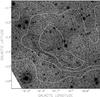 |
Fig. 3 Cutout of the bright radio shell of G190.9−2.2 corresponding to the box outlined on the 21 cm panel of Fig. 2, showing optical (red) emission from the Second Palomar Observatory Sky Survey (bright emission is shaded dark here). A thin compressed filament of red nebulosity is seen running parallel and next to the innermost 21 cm radio contour, which is the completely enclosed white contour in the centre (the three white contours here are the same as are in the 21 cm panel of Fig. 2). This filament likely traces shocked gas downstream of the SNR shock. |
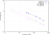 |
Fig. 4 Integrated radio flux spectra for each object, and overlaid power-law fitted with least squares weighted by uncertainties. For G190.9−2.2 the spectrum with index α4 is calculated over 408 MHz–4.8 GHz (λ74−6 cm) only and does not include the 30.9 MHz flux point from Kassim (1988). |
The PI map at 6 cm (Fig. 2) shows the eastern shell to be 30−50% polarized, but the other parts of the SNR candidate seem to be unpolarized. This could be the result of the low surface brightness combined with uncertain contributions from the unrelated interstellar medium along the line-of-sight. The B-vectors derived for the eastern shell indicate a tangential magnetic field which would be expected for a mature shell-type remnant. This provides further evidence that G190.9−2.2 is a supernova remnant.
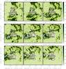 |
Fig. 5 12CO line channel maps towards G152.4−2.1. The brightness scale is antenna temperature TA in K, and the angular resolution of the maps is 1′. Three thick white-on-black contours traced at 100, 130 and 160 mK delineate the total power appearance of G152.4−2.1 at 21 cm. Overlaid on each map are thick pure white contours that outline HISA clouds seen in CGPS H i maps at the same velocities. A single TB = 90 K contour (very thin black) outlines the brightest H i cloud in the field, appearing in between the molecular clouds that follow the outside of the southern shell. All of this activity peaks at vLSR = −12 km s-1. |
3.3. Integrated flux densities
Integrated flux densities are summarized in Table 1. Tabulated fluxes are averages obtained over 20 polygons each with two kinds of background surfaces fitted to the data values at the polygon vertices: twisted-plane and twisted-quadratic surfaces. Twisted plane surfaces have the property that orthogonal cuts through them at one particular rotation angle are linear, and twisted quadratics have one orientation in which all cuts through the surface are linear, and all orthogonal cuts are quadratic. Uncertainties in fluxes (ΔS) accumulate from three sources: i) the uncertainty in the total intensity calibration of each map (±4, 10, 5, 15 and 20% for λ = 6, 11, 21, 74, and 92 cm respectively); ii) the deviation in the background-subtracted flux over different polygons enclosing the emission (drawn by eye); and iii) the mean difference in background flux levels estimated with both types of background surface fits. A linear fit of log S versus logν was calculated with least squares weighted by ΔS. Each object shows a steep power-law radio spectrum identifying the integrated emission as non-thermal (see Fig. 4). For G152.4−2.1 the integrated spectral index is α = −0.65 ± 0.05 (Sν ∝ να).
Integrated flux and spectral properties of G152.4−2.1 and G190.9−2.2 from point-source-subtracted Stokes I maps at five radio frequencies.
For G190.9−2.2 α = −0.66 ± 0.05 (without the 30.9 MHz flux point of Kassim (1988)α = −0.59 ± 0.14). Also reported in Table 1 is each object’s estimated flux density and surface brightness at 1 GHz, the mean centroid coordinates, and the major and minor angular diameters and orientation angle of each shell (fitted by eye). At 1 GHz the surface-brightness of both SNRs (as listed in Table 1) would make them the faintest yet catalogued, below the previous faintest SNR G156.2+5.7 (5.8×10⁻²³ W m-2 Hz-1 sr-1; Reich et al. 1992).
4. HI and CO velocities and distances
We determine systemic LSR velocities for both SNRs along their lines-of-sight using ~1′ resolution CGPS 21 cm H i line data and 45″ resolution 2.6 mm (115.3 GHz) 12CO(J = 1 → 0) line data from the Exeter FCRAO CO Galactic Plane Survey (described in Mottram & Brunt 2010; Brunt et al. 2012).
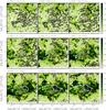 |
Fig. 6 12CO line channel maps towards G190.9−2.2. The brightness scale is antenna temperature TA in K, and the resolution 1′. Three thick white-on-black contours traced at 100, 150 and 200 mK delineate the total power appearance of G152.4−2.1 at 21 cm. Extended HISA is contoured with thick pure white lines (level −20 K below the mean TB level of each H i channel), and H i emission at 6 and 9 Kelvin (above the mean of each map) is shown with the thin black contours. In channels with vLSR = +4.3 and 5.1 km s-1 molecular gas is seen bracketing the SNR’s east and west boundaries, and curved shell-like atomic gas clouds bracket the north and south boundaries. |
Figure 5 is a 9-channel montage of 12CO and H i towards G152.4−2.1. Each channel is spaced to 0.82 km s-1 and the velocity resolution is 1.32 km s-1. The CO maps have been smoothed to 1′ spatial resolution to match the H i. In all velocity channels, line emission towards G152.4−2.1 shows no obvious cavity nor shell of neutral or molecular gas surrounding it (as an SNR evolving in a stellar wind bubble might; e.g. 3C 434.1, Foster et al. 2004). Rather, the continuum boundary is sharply delimited by a wall of bright CO that systematically wraps the eastern boundary of the SNR from the south to the north. This bright CO (TA = 1−2 K) emission begins outside of the southern shell boundary at vLSR = −8.9 km s-1 and in each of the following channels (−10.5 to −13 km s-1) the CO neatly matches the curvature of the sharp southeast corner of the shell. Also tracing the SNR’s southeast and east periphery are numerous H i self-absorption (HISA) clouds (white contours in Fig. 5) in CGPS maps at the same velocities. The CO and HISA environment seems to form a “wall” of cool dense gas on the sky next to the east continuum boundary of the SNR. As well, CO and HISA appear to neatly fill in an eastern “bay” formed by the continuum contours at  ,
,  . An isolated bright cloud of H i emission (single 90 K thin black contour in each map of figure), the brightest such cloud in the entire field and the only H i emission feature possibly associated with the SNR, is seen exactly in the gap between the CO clouds that wrap along the outside of the southern shell, at ,
  . All of these spatial coincidences occur in nine channels between −8.9 and −15.5 km s-1. Their spatial relation with respect to the shell is similar in channels −10.5 to −13 km s-1, suggesting a systemic velocity of vLSR ≃ −12 ± 2 km s-1 for G152.4−2.1.
Figure 6 is a 9-channel montage of 12CO and H i centred on G190.9−2.2. Two bright CO clouds that begin to appear at +6.0 km s-1 flank the SNR on its left (east) and right (west) sides. This relationship is particularly striking in channels from +5.1 to +3.5 km s-1 where the CO clouds are dense and bright and continue to flank the SNR’s east and west continuum boundary. At the same velocities an extensive HISA cloud that well traces the outline of the CO cloud in the east appears, and another HISA cloud just begins to appear atop the western CO at +3.5 km s-1. In later channels vLSR ≤ 2.7 km s-1 this CO+HISA appears atop the SNR’s face, suggesting it is in front or behind it and sporting little relation with the continuum appearance. H i emission surrounding G190.9−2.2 is much more complex than seen towards G152.4−2.1, and appears in the same velocity channels as the CO but in the opposite corners: above and below the object’s north and south boundaries respectively. Both of these north and south H i “caps” follow the curvature of the SNR’s limb at 21 cm in four channels +7.6−+5.1 km s-1; thereafter the north arc disappears and the south has grown into a large H i wall off of the south southwest corner of the SNR. The overall appearance of G190.9−2.2 being nestled within CO+HISA walls to the east and west and H i emission shells to its north and south is particularly striking in the channel map at vLSR = +5.1 ± 1.6 km s-1. Based on this appearance we assign this as the systemic velocity of G190.9−2.2.
Even with a systemic velocity in hand, ascribing distances to these two objects is not straightforward. Under undisturbed circular rotation vLSR = −12 ± 2 km s-1 places G152.4−2.1 within the “Local arm” at a distance of ~1.1 ± 0.1 kpc (using the rotation curve of Foster & Cooper 2010). This SNR then has a linear diameter of 32 × 30 pc. The gradient Δr/ΔvLSR here is 110 pc per km s-1, which gives the minimum uncertainty. However the association with HISA implies that neutral hydrogen at two different distances is present in these velocity channels (i.e. a cold foreground and a warm background), showing that circular rotation in this direction is anything but undisturbed and that the error on the distance is expected to be greater.
A kinematic distance to G190.9−2.2 of 1.0 ± 0.3 kpc is indicated based on the CO+H i-based velocity of +5.1 km s-1, implying physical dimensions of 18 × 16 pc. The uncertainty in this distance is large however, as the 1/sin ℓ projection here causes a small velocity range to represent a large line-of-sight path, and small velocity deviations from circular rotation are magnified into large distance uncertainties (here Δr/ΔvLSR ~ 200 pc per km s-1). We know such deviations are present as remarkable and extended HISA is seen through the field, so again the distance error is a lower limit.
5. Conclusion and future
The purpose of this paper is twofold. Firstly we introduce two extended faint discrete objects discovered in the CGPS and show evidence (mainly through their radio spectral and polarization properties) that classifies them as SNRs. Secondly we provide a basic qualitative interpretation and quantitative physical properties (fluxes, distances, sizes) that will aid the community in planning future new observations of them at radio and especially other wavelengths (e.g. X-ray, optical). The objects were discovered by deep point source subtraction (down to 2σ level) and subsequent smoothing of two selected CGPS 21 cm continuum mosaics, to increase the S/N of faint extended emission. Their identity as SNRs was then discovered spectrally through comparison with other wavelengths (e.g. 74 cm component of the CGPS; the Sino-German 6 cm polarization survey). Undoubtedly many more such extended low surface brightness SNRs await discovery within this rich dataset using
this approach. Such discoveries will further address the “missing SNR” problem that is a key driver of new and planned deep radio surveys of the Milky Way’s ISM.
Available at http://www3.mpifr-bonn.mpg.de/survey.html
Acknowledgments
We thank the referee for their thorough reading of our manuscript and the many thoughtful suggestions they provided. We would also like to thank Chris Brunt (Exeter) for providing the CO data, and Dr. JinLin Han and Dr. Xuyang Gao (NAOC) for providing the 6 cm data prior to its public release. The Dominion Radio Astrophysical Observatory is a National Facility operated by the National Research Council. The Canadian Galactic Plane Survey is a Canadian project with international partners, and is supported by the Natural Sciences and Engineering Research Council (NSERC). The discovery of G190.9−2.2 by BC was made possible by a Brandon University Research Committee (BURC) grant to T.F. The discoveries described here were made in part based on observations with the 100-m telescope of the MPIfR (Max-Planck-Institut für Radioastronomie) at Effelsberg.
References
- Brogan, C. L., Gelfand, J. D., Gaensler, B. M., Kassim, N. E., & Lazio, T. J. W. 2006, ApJ, 639, L25 [NASA ADS] [CrossRef] [Google Scholar]
- Brunt, C. M., Heyer, M., Mottram, J. C., Douglas, K. A., & Summers, L. 2012, in prep. [Google Scholar]
- Caswell, J. L. 1977, Proc. Astron. Soc. Aust., 3, 130 [NASA ADS] [Google Scholar]
- Emerson, D. T., & Graeve, R. 1988, A&A, 190, 353 [NASA ADS] [Google Scholar]
- Ferrand, G., & Safi-Harb, S. 2012, Adv. Space Res., 49, 1313 [NASA ADS] [CrossRef] [Google Scholar]
- Finkbeiner, D. P. 2003, ApJS, 146, 407 [NASA ADS] [CrossRef] [Google Scholar]
- Foster, T., & Cooper, B. 2010, in The Dynamic Interstellar Medium: A Celebration of the Canadian Galactic Plane Survey, eds. R. Kothes, T. L. Landecker, & A. G. Willis (San Francisco, CA: ASP), ASP Conf. Ser., 438, 16 [Google Scholar]
- Foster, T., Routledge, D., & Kothes, R. 2004, A&A, 417, 79 [NASA ADS] [CrossRef] [EDP Sciences] [Google Scholar]
- Frail, D. A., Goss, W. M., & Whiteoak, J. B. Z. 1994, ApJ, 437, 781 [NASA ADS] [CrossRef] [Google Scholar]
- Fürst, E., Reich, W., Reich, P., & Reif, K. 1990, A&AS, 85, 691 [NASA ADS] [Google Scholar]
- Gaensler, B. M. 1998, ApJ, 493, 781 [NASA ADS] [CrossRef] [Google Scholar]
- Gao, X. Y., Reich, W., Han, J. L., et al. 2010, A&A, 515, A64 [NASA ADS] [CrossRef] [EDP Sciences] [Google Scholar]
- Gao, X. Y., Sun, X. H., Han, J. L., et al. 2011, A&A, 532, A144 [NASA ADS] [CrossRef] [EDP Sciences] [Google Scholar]
- Green, D. A. 2009, Bull. Astron. Soc. India, 37, 45 (also available at http://www.mrao.cam.ac.uk/surveys/snrs) [Google Scholar]
- Green, D. A. 2011, Bull. Astron. Soc. India, 39, 289 [Google Scholar]
- Haslam, C. G. T. 1974, A&AS, 15, 333 [NASA ADS] [Google Scholar]
- Higgs, L. A., Hoffmann, A. P., & Willis, A. G. 1997, in Astronomical Data Analysis Software and Systems VI, eds. G. Hunt, & H. Payne, ASP Conf. Ser., 125, 58 [Google Scholar]
- Kassim, N. E. 1988, A&AS, 68, 715 [Google Scholar]
- Kerton, C. R., Murphy, J., & Patterson, J. 2007, MNRAS, 379, 289 [NASA ADS] [CrossRef] [Google Scholar]
- Koo, B.-C., Kang, J.-H., & Salter, C. J. 2006, ApJ, 643, 49 [Google Scholar]
- Kothes, R. 2003, A&A, 408, 187 [NASA ADS] [CrossRef] [EDP Sciences] [Google Scholar]
- Kothes, R., Landecker, T. L., Foster, T., & Leahy, D. A. 2001, A&A, 376, 641 [NASA ADS] [CrossRef] [EDP Sciences] [Google Scholar]
- Kothes, R., Uyanıker, B., & Reid, R. 2005, A&A, 444, 871 [NASA ADS] [CrossRef] [EDP Sciences] [Google Scholar]
- Kothes, R., Fedotov, K., Foster, T. J., & Uyanker, B. 2006, A&A, 457, 1081 [NASA ADS] [CrossRef] [EDP Sciences] [Google Scholar]
- Landecker, T. L., Reich, W., Reid, R. I., et al. 2010, A&A, 520, A80 [NASA ADS] [CrossRef] [EDP Sciences] [Google Scholar]
- Li, Z., Wheeler, J. C., Bash, F. N., & Jefferys, W. H. 1991, ApJ, 378, 93 [NASA ADS] [CrossRef] [Google Scholar]
- Manchester, R. N. 1987, A&A, 171, 205 [NASA ADS] [Google Scholar]
- Mottram, J. C., & Brunt, C. M. 2010, in The Dynamic Interstellar Medium: A Celebration of the Canadian Galactic Plane Survey, eds. R. Kothes, T. L. Landecker, & A. G. Willis (San Francisco, CA: ASP), ASP Conf. Ser., 438, 98 [Google Scholar]
- Reich, W., Fürst, E., Haslam, C. G. T., Steffen, P., & Reif, K. 1984, A&AS, 58, 197 [NASA ADS] [Google Scholar]
- Reich, W., Fürst, E., & Arnal, E. M. 1992, A&A, 256, 214 [NASA ADS] [Google Scholar]
- Rengelink, R. B., Tang, Y., de Bruyn, A. G., et al. 1997, A&AS, 124, 259 [NASA ADS] [CrossRef] [EDP Sciences] [Google Scholar]
- Sofue, Y., & Reich, W. 1979, A&AS, 38, 251 [NASA ADS] [Google Scholar]
- Spoelstra, T. A. T. 1984, A&A, 135, 238 [NASA ADS] [Google Scholar]
- Sun, X. H., Han, J. L., Reich, W., et al. 2007, A&A, 463, 993 [NASA ADS] [CrossRef] [EDP Sciences] [Google Scholar]
- Taylor, A. R., Gibson, S. J., Peracaula, M., et al. 2003, AJ, 124, 3145 [NASA ADS] [CrossRef] [Google Scholar]
- Tian, W. W., Leahy, D. A., & Foster, T. J. 2007, A&A, 465, 907 [NASA ADS] [CrossRef] [EDP Sciences] [Google Scholar]
All Tables
Integrated flux and spectral properties of G152.4−2.1 and G190.9−2.2 from point-source-subtracted Stokes I maps at five radio frequencies.
All Figures
|
Fig. 1 Total (I) and polarized intensity (PI) contoured maps of G152.4−2.1. The emission features (colour bars in brightness temperature units of K, at right) are themselves outlined in thin black contours (levels indicated in the text above each panel). B-field vectors are overlaid on PI maps (length proportional to PI; scale differs between maps). Resolutions are 9 |
| In the text | |
|
Fig. 2 Total (I) and polarized intensity (PI) contoured maps of G190.9−2.2. The emission features (colour bars in brightness temperature units of K, at right) are themselves outlined in thin black contours (levels indicated in the text above each panel). B-field vectors are overlaid on PI maps (length proportional to PI; scale differs between maps). Resolutions are 9 |
| In the text | |
|
Fig. 3 Cutout of the bright radio shell of G190.9−2.2 corresponding to the box outlined on the 21 cm panel of Fig. 2, showing optical (red) emission from the Second Palomar Observatory Sky Survey (bright emission is shaded dark here). A thin compressed filament of red nebulosity is seen running parallel and next to the innermost 21 cm radio contour, which is the completely enclosed white contour in the centre (the three white contours here are the same as are in the 21 cm panel of Fig. 2). This filament likely traces shocked gas downstream of the SNR shock. |
| In the text | |
|
Fig. 4 Integrated radio flux spectra for each object, and overlaid power-law fitted with least squares weighted by uncertainties. For G190.9−2.2 the spectrum with index α4 is calculated over 408 MHz–4.8 GHz (λ74−6 cm) only and does not include the 30.9 MHz flux point from Kassim (1988). |
| In the text | |
|
Fig. 5 12CO line channel maps towards G152.4−2.1. The brightness scale is antenna temperature TA in K, and the angular resolution of the maps is 1′. Three thick white-on-black contours traced at 100, 130 and 160 mK delineate the total power appearance of G152.4−2.1 at 21 cm. Overlaid on each map are thick pure white contours that outline HISA clouds seen in CGPS H i maps at the same velocities. A single TB = 90 K contour (very thin black) outlines the brightest H i cloud in the field, appearing in between the molecular clouds that follow the outside of the southern shell. All of this activity peaks at vLSR = −12 km s-1. |
| In the text | |
|
Fig. 6 12CO line channel maps towards G190.9−2.2. The brightness scale is antenna temperature TA in K, and the resolution 1′. Three thick white-on-black contours traced at 100, 150 and 200 mK delineate the total power appearance of G152.4−2.1 at 21 cm. Extended HISA is contoured with thick pure white lines (level −20 K below the mean TB level of each H i channel), and H i emission at 6 and 9 Kelvin (above the mean of each map) is shown with the thin black contours. In channels with vLSR = +4.3 and 5.1 km s-1 molecular gas is seen bracketing the SNR’s east and west boundaries, and curved shell-like atomic gas clouds bracket the north and south boundaries. |
| In the text | |
Current usage metrics show cumulative count of Article Views (full-text article views including HTML views, PDF and ePub downloads, according to the available data) and Abstracts Views on Vision4Press platform.
Data correspond to usage on the plateform after 2015. The current usage metrics is available 48-96 hours after online publication and is updated daily on week days.
Initial download of the metrics may take a while.