| Issue |
A&A
Volume 556, August 2013
|
|
|---|---|---|
| Article Number | A130 | |
| Number of page(s) | 13 | |
| Section | Astrophysical processes | |
| DOI | https://doi.org/10.1051/0004-6361/201219901 | |
| Published online | 05 September 2013 | |
The creation of photonic orbital angular momentum in electromagnetic waves propagating through turbulence⋆,⋆⋆,⋆⋆⋆
1 Air Force Research Laboratory, Directed Energy Directorate, Kirtland AFB, New Mexico, USA
e-mail: This email address is being protected from spambots. You need JavaScript enabled to view it.
2 Science Applications International Corporation, Albuquerque, New Mexico, USA
Received: 26 June 2012
Accepted: 12 May 2013
Abstract
Context. We have recently shown that the phenomenon known as “branch points” in AO are markers for photons carrying orbital angular momentum (OAM). In doing so, we have demonstrated that atmospheric turbulence creates well defined OAM states in beams propagating through it.
Aims. In this paper, we extend our previous research to include any astrophysical turbulent assemblage of molecules or atoms (TAMA), demonstrating that these clouds, similar to Earth’s atmosphere, also create photonic orbital angular momentum (POAM) in electromagnetic waves propagating through them. A TAMA is any gaseous cloud with a varying density and therefore variation in its index of refraction, which includes but is not limited to stellar envelopes, circumstellar disks, molecular clouds, planetary atmospheres, and the interstellar medium.
Methods. We applied our previous theoretical, simulation, and laboratory results to astrophysical TAMAs. Additionally, we demonstrated how sensors designed for AO can be used to measure this POAM flux.
Results. Our results apply to light propagating through any TAMA. Since TAMA are ubiquitous in the cosmos, steady, long lasting POAM fluxes will be ubiquitous as well.
Conclusions. Our results, which include theory, benchtop laboratory data, and wave optic simulation, indicate that, under the right conditions, POAM fluxes can reach over 50% of the total photon flux. An initial set of on-sky experimental observations appear to corroborate the laboratory results with two of the five stars, HR 1529 and HR 1577, showing POAM fluxes of 3% ± 1% and 2% ± 1% of the total flux, and a third, HR 1895, with a PAOM flux of up to 17% ± 2% of the total flux.
Key words: instrumentation: adaptive optics / turbulence / waves / radiation mechanisms: general / ISM: clouds
We express our gratitude to the Air Force Office of Scientific Research for their support of this research.
Appendices are available in electronic form at http://www.aanda.org
Data referred to in measurements are only available at the CDS via anonymous ftp to cdsarc.u-strasbg.fr (130.79.128.5) or via http://cdsarc.u-strasbg.fr/viz-bin/qcat?J/A+A/556/A130
© ESO, 2013
1. Introduction
Recent work has shown that orbital angular momentum (OAM) can be carried by electromagnetic fields from the radio to optical to X-rays (Mohammadi et al. 2010; Allen et al. 1992; Peele et al. 2002), as well as by electrons (Hemsing et al. 2012) and quarks (Chen et al. 2008; Tao et al. 2011). For our part, we have recently demonstrated that photons with OAM are created by propagation through atmospheric turbulence (Sanchez & Oesch 2011a,b). In this work, we extend our result and demonstrate that photonic orbital angular momentum (POAM) is created as a natural consequence of electromagnetic waves propagating through any astrophysical turbulent assemblage of molecules or atoms (TAMA) and that this creates steady and long-lasting POAM fluxes.
The basis of our treatment is (1) to demonstrate that the physical requirements for the creation of POAM in Earth’s atmosphere are present in astrophysical TAMAs; and (2) to demonstrate that the POAM flux created by TAMAs can be measured. Demonstration of the first is a straightforward application of our previous results. Demonstration of the second is more demanding. Whereas observation of astronomical sources relies on measurement of the intensity, wavelength, polarization, or coherence (imaging) of electromagnetic waves to interrogate remote physical systems, for instance gravitational interactions from images, none use the recently enumerated property of POAM (Uribe-Patarroyo et al. 2011). We present the first such observations in Sect. 4.
There is recognition in the community that measurement of POAM would be useful. Harwit (2003) proposed why measurement of OAM could be of use in astrophysical observations. Later, Elias (2008, 2012) both surveyed the role POAM could play in astronomical observations and also proposed a framework for future research to include how measurements of POAM would interact with more conventional astronomical instrumentation (Elias 2012). However, no prior work enumerates a mechanism by which POAM can be widespread in the cosmos. We present such a mechanism in Sect. 3.
Whereas no prior measurement of astrophysical POAM has been attempted, a few works detail specific examples of the formation or use of POAM in astronomy or new instrumentation for its detection. For example, Tamburini et al. (2011) found that photons could be imparted with orbital angular momentum through interaction with a Kerr black hole. Also, Uribe-Patarroyo et al. (2011) discuss solar photons carrying orbital angular momentum and their use in comparing properties of different solar regions. Berkhout & Beijersbergen (2009, 2010) discussed use of a multipoint interferometer as a method of identifying optical vortices in astronomical sources and elsewhere (Berkhout et al. 2011) described an optical system utilizing two custom optical components for detection of multiple OAM modes simultaneously. Lavery et al. (2011) presented a geometric transformation as an approach to analyze the superposition of OAM states.
The first description of POAM was given by Jackson (1975). Later, Allen et al. (1992) demonstrated that photons in a Laguerre-Gaussian (L-G) beam carry mħ of OAM where m denotes the mth OAM state, and that this beam can be created as a conversion process from a non-OAM carrying Hermite-Gaussian (H-G) beam through the use of cylindrical lenses. Sanchez & Oesch (2011a) demonstrated that smooth, but random turbulence, also acts as a conversion process which converts non-OAM to OAM photons.
In Earth’s atmosphere, optical turbulence is caused by index of refraction fluctuations which in turn are caused by density fluctuations. Density fluctuations are induced by contra-velocity flows, which are mostly due to diurnal heating. The contra-velocity flows cause eddies. These eddies cascade to smaller and smaller scales until molecular collision becomes important, at which time viscous dissipation occurs (Andrews & Phillips 1998). The characteristic length at which this occurs is called the inner scale of turbulence. The size of the inner scale of turbulence strongly influences both scintillation (Hill & Ochs 1992) and also creation of POAM (Sanchez & Oesch 2011b). The strength of the density fluctuations is characterized by the structure function of the index of refraction, with the quasi-equilibrium state described by a Kolmogorov structure function (Andrews & Phillips 1998).
The amount of turbulence-induced POAM has been shown to vary based on turbulence strength and propagation distance (Sanchez & Oesch 2011b). This is fundamentally different than in the conversion of H-G beams to L-G beams, because, in that case, all photons in the H-G beam are converted from m = 0 to the m ≠ 0 state. In the turbulence conversion process, only a fraction of the total photon flux is converted to a POAM flux. In Sect. 4, we demonstrate to first order that this flux can reach over half of the total flux (Sanchez & Oesch 2012).
POAM can be measured using a Shack-Hartmann wavefront sensor (Leach et al. 2006; Murphy et al. 2010), similar to those used in conventional adaptive optical (AO) systems. Shack-Hartmann wavefront sensors (SH WFS) measure the gradient of a beam’s phase, ∇ϕ. The phase can be separated into two parts, the rotational phase, ϕRot, which contains the phase of the non-zero POAM carrying photons, and the least mean square phase, ∇ϕLMS, which carries zero POAM. Note however, even though SH WFSs measure the total phase, and hence the POAM component of the beam, in standard AO processing, in order to reduce noise, ϕRot is discarded in the reconstruction process (Fried 1998). This means that using standard techniques, the POAM component of the beam is overlooked, but with special processing, can be extracted. More on this in Sects. 2 and 4.
The primary purpose of this paper is to demonstrate that propagation through TAMAs creates POAM and the created POAM flux can be measured. The secondary purpose is to present the first on-sky measurements of astrophysical POAM flux. To this end, Sect. 2 reviews previous results, interactions of POAM with matter, and characterizations of atmospheric turbulence. Then, Sect. 3 reviews the physical mechanism by which astrophysical TAMAs create POAM. A first order calculation of the magnitude of the POAM flux is given in Sect. 4. Then, on-sky observations are presented in Sect. 5 followed by a summary in Sect. 6.
2. Background
The basis of the demonstration rests directly on classic AO theory. Adaptive optics (Fugate et al. 1991) was created to mitigate atmospheric turbulence and, in doing so, produced major results in both understanding turbulence as a physical process, as well as, measurement of that turbulence; we use both here.
2.1. Adaptive optics and the two types of phase
In the presence of atmospheric turbulence, an optimal phase for image formation exists; call it ϕLMS. Fried (1998) demonstrated that the gradient of the phase is uniquely comprised of two constituents, ∇ϕLMS and ∇ϕRot and hence the phase is comprised of two components, the optimal phase for image formation, ϕLMS, and a discontinuous phase, ϕRot, caused by branch points, i.e.  (1)Brennan (priv. comm., TR-1648) later demonstrated that the phase gradients exist in two orthogonal Hilbert spaces, ℋLMS and ℋrot, such that
  (2)with the Hilbert spaces corresponding, respectively, to the phases in Eq. (1). The phase gradients can be identified with these Hilbert spaces via projection operators,
  and
and  , i.e.
  and
and  . (For a discussion of the projection operators, see Appendix A.)
Branch points can be measured (Fried & Vaughn 1992; Fried 1998) by summing the phase in closed contours. A result of ± 2π indicates the presence of a branch point within the contour. In the case of the gradients returned by Shack-Hartmann wavefront sensors,  (3)signifies the presence of a branch point with Ωi a closed contour along the discrete samples, and ri the location of the ith wavefront sensor subaperture.
2.2. The discarding of the rotational phase by astronomical AO systems
Adaptive optic systems compensate for turbulence by measuring phase gradients, reconstructing the measured gradients into phase, then, through a control law, turning the reconstructed phase into deformable mirror commands. Observing near zenith, it can be shown that ϕRot = 0, that is, ϕ = ϕLMS. Hence, in an AO system measurement of the phase, all components of the gradients in ϕRot are noise, and as such, are discarded by the AO phase reconstructors. See Appendix A for more comprehensive discussion of this point.
2.3. The morphology of branch points
Atmospheric turbulence is a continuous, thin disturbance making ϕRot = 0 at the disturbance, which implies there are no branch points at the disturbance. Branch points are created with additional propagation.
2.3.1. Creation pairs
Branch points are created infinitesimally close together in pairs of opposite helicity (Sanchez & Oesch 2009). As the wave propagates, the pairs drift apart (Oesch et al. 2012d). As such, there is a natural geometry associated with creation pairs (Sanchez et al. 2010) given by their inter-pair separation, call it Δ, and their intra-pair separation, call it δ. This geometry is depicted in Fig. 1b where the natural geometry for creation pairs is depicted in sample simulation data with overlay of Δ and δ. The phase of a single branch point, if it could exist in nature, is shown in Fig. 1a, but this is also the phase for the m = 1 Laguerre-Gaussian beam. Figure 2 plots this for two sample experimental data sets, a low branch point density case on the left with δ ≪ Δ and a high density case on the right with δ < Δ.
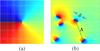 |
Fig. 1 a) Phase of a single branch point, if it could exist in nature. Also, the phase for the m = 1 Laguerre-Gaussian beam which is known to rapidly decohere in the presence of turbulence. b) ϕRot for a distribution of creation pairs with an overlay of Δ and δ. The scale on both plots is [− π,π]. |
2.3.2. Δ and δ
Branch point density is inversely proportional to Δ but is very much easier to measure and hence is the experimentalist’s parameter of choice. Oesch et al. (2012d) measured branch point density as a function of propagation distance. He found that branch points are formed only after some distance, call it z0, then their density increases as the 11/6th power of normalized propagation distance until some distance, call it zss, at which it begins to deviate from z11/6. With additional propagation, the density climbs reaching its maximum value at zρmax, then decreases thereafter. In the unsaturated regime, an empirical form of the density is found to be  (4)Similarly, the intra-pair separation is found to be
  (5)Experimental measurement (Oesch et al. 2012d) for these two parameters is shown in Fig. 3 with intra-pair separation shown on the left and the inverse of inter-pair separation shown on the right.
Note that when ρBP is low and δ is small, φRot is highly localized. This is readily apparent in Fig. 2a.
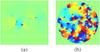 |
Fig. 2 Experimental data of ϕRot, a) low branch point density, b) high branch point density. The scale on both plots is [− π,π]. |
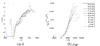 |
Fig. 3 ASALT laboratory data highlighting creation pair behavior. Eleven values of turbulence strength with r0 in the range 6.5 − 16.6 cm. a) Intra-pair separation as a function of normalized distance. b) The inverse of the inter-pair separation, i.e. branch point density, as a function of propagation distance. |
2.3.3. Wavelength dependence
Our research has been conducted at optical and near IR wavelengths. Specifically, our laboratory data (Oesch et al. 2010, 2012d; Oesch & Sanchez 2012) is at 1.55 microns. Most of our simulation data (Oesch et al. 2012d) is also at 1.55 microns. Our recent field data (Farrell et al. 2012; Oesch et al. 2013a,b) is in the red, 633 nm for our 3 Km tests and approximately 600 nm for our 50 m tests. The on-sky data presented in Sect. 5 is taken at 450 − 650 nm. The theoretical work which rests on the laboratory data and wave optics simulation (Sanchez et al. 2010, 2012) also adhere to those wavelengths. The theoretical work which links turbulence, via branch points, to the creation of POAM (Sanchez & Oesch 2011a,b) is applicable throughout the visible. The foundational work (Sanchez & Oesch 2009), which proved that branch points are created in pairs of opposite helicity and opened the door for the study of branch points as enduring features of the traveling wave, relies only on causality, and hence is independent of wavelength. In a similar vein, Elias (2012) demonstrated that pairs of opposite helicity are created by astronomical sources on the celestial sphere. In AO, the earliest works that studied branch points (Fried & Vaughn 1992; Fried 1998) are applicable from visible wavelengths to the near infrared. POAM itself has been found in electromagnetic radiation from radio waves (Mohammadi et al. 2010) to x-rays (Peele et al. 2002).
2.4. Turbulence
Up to this point, we have casually used the word turbulence. Here we define it, with special emphasis on two parameters of interest, strength and inner scale.
2.4.1. The structure function of turbulence
Optical turbulence in a gaseous cloud is caused by fluctuations in the index of refraction which, in turn, is caused by density fluctuations. The structure function of index fluctuations quantifies turbulence strength (Sasiela 2007; Andrews & Phillips 1998) ![Mathematical equation: \begin{eqnarray} \label{eq: structure function} \mathcal{D}(\bfr) = \left< \left[ n(\epsilon(a)) - n(\epsilon(a+\bfr)) \right]^2 \right> \end{eqnarray}](/articles/aa/full_html/2013/08/aa19901-12/aa19901-12-eq53.png) (6)where n(·) is the index of refraction with its explicit dependence of the permittivity, ϵ(r), shown and r is the spatial coordinate. The structure function is comprised of an inertial range bounded above and below by the outer and inner scales of turbulence, respectively. The outer scale, L0, denotes the largest coherent structure in the turbulence. The inner scale, l0, is the characteristic length at which bulk motion is dissipated as heat. A TAMA, then, is any assemblage of molecules or atoms in which
(6)where n(·) is the index of refraction with its explicit dependence of the permittivity, ϵ(r), shown and r is the spatial coordinate. The structure function is comprised of an inertial range bounded above and below by the outer and inner scales of turbulence, respectively. The outer scale, L0, denotes the largest coherent structure in the turbulence. The inner scale, l0, is the characteristic length at which bulk motion is dissipated as heat. A TAMA, then, is any assemblage of molecules or atoms in which  is not constant.
Considering the special case of variations in for which the gas is in quasi-equilibrium and accounting for both l0 and L0, Eq. (6) reduces to  (7)The regime where l0 < r < L0 is known as the inertial subrange of turbulence. A power spectrum can be calculated for Eq. (7), and is given by the von Karman spectrum
  with
with  the inner scale (in frequency) of turbulence,
  the outer scale (in frequency). With regards to optical propagation, the inner scale is the highest frequency at which turbulence structures are supported. Turbulence spectra with an 11/3 dependence in the inertial subrange are known as Kolmogorov spectra. Also note, TAMAs need not be in quasi-equilibrium; we present the Kolmogorov spectrum because it is widely used and facilitates calculation.
2.4.2. Turbulence strength
In Kolmogorov’s structure function model of atmospheric turbulence, turbulence strength is simply  in Eq. (7). Unfortunately, must be measured in-situ which, for astrophysical TAMAs, is problematic. Hence, two other measures, calculable from the propagating beam, are commonly used to infer turbulence strength, both of which are based on the Rytov approximation and a Kolmogorov spectrum (Sasiela 2007; Andrews & Phillips 1998).
The first is Fried’s parameter, r0, which is an estimate of phase variation in the beam. Theoretically, Fried’s parameter is proportional to the zeroth moment of (Sasiela 2007), i.e.  (8)Experimentally, Fried’s parameter can be estimated from wavefront sensor data, which in the case of the gradients measured by a Shack-Hartmann wavefront sensor, is given by (Brennan & Mann 2010)
  (9)where d is the subaperture size and
  is the variance of the wavefront sensor gradients.
The second common estimate of turbulence strength is Rytov’s parameter,  , which is an estimate of scintillation in the beam. Theoretically, Rytov’s parameter is proportional to the 5/6th propagation moment of (Sasiela 2007), i.e.
  (10)Experimentally, Rytov’s parameter cannot be directly measured, but can be inferred from the scintillation index (Andrews & Phillips 1998)
  (11)where I is the intensity,
  the variance of intensity, and ⟨I⟩ the mean. At low scintillation,
  .
.
2.4.3. The inner scale of turbulence
The inner scale of turbulence is the characteristic length at which bulk velocity is converted to heat. In this sense, it is a thermodynamic quantity.
There are relatively few measurements of the inner scale compared to the number of measurements of r0, although recently Farrell et al. (2012), Brennan & Mann (2010) have published measurements of the inner scale at low altitude in daylight including means to estimate the inner scale using propagating beam parameters. They found l0 = 1 − 5 mm.
There are no known measurements of the inner scale for astrophysical TAMAs. So, even though it is central to exact calculation of branch point creation, dearth of measurement and calculation leads us to proceed in the remainder of the paper with the benign assumption that inner scale is finite in astrophysical TAMAs.
In AO applications, ϕRot = 0, and turbulence strength equates directly to Fried’s parameter. However, under extended propagation, Oesch et al. (2012d) demonstrated that the inner scale of turbulence has as large an impact on branch point creation as . Interestingly, this observation ties branch point formation to a thermodynamic property of the TAMA.
2.5. Turbulence-induced POAM
Jackson (1975) noted for a traveling wave with electric and magnetic components, E and B, respectively, and transverse spatial coordinates r, that r × E × B ≠ 0 is sufficient to indicate the existence of POAM. This implies a component of the field in the direction of propagation. The component of the electric field in the direction of propagation causes the instantaneous Poynting vector to spiral about the direction of propagation, and leads to 2π circulations in phase. The electric field then has the characteristic proportionality of  (12)with m an integer and ϕ the azimuthal coordinate.
Allen et al. (1992) demonstrated both that POAM can be carried by L-G beams and that these beams can be easily created in the laboratory by conversion of H-G beams. The conversion takes place by propagating through two cylindrical lenses, and note that the phase imparted by the cylindrical lenses is smooth. Sanchez & Oesch (2011a,b) and Oesch et al. (2012b) have demonstrated that atmospheric turbulence is also a conversion process, creating non-zero POAM, although unlike the cylindrical lenses in the H-G to L-G conversion, the conversion here is spatially localized.
Two notes in passing. First, the type of turbulence spectrum, e.g. Kolmogorov, is irrelevant to whether POAM is created. The type of spectrum does, however, affect both z0 and ρ, and an assumption of a Kolmogorov spectrum is useful in that it allows for calculation. Secondly, the atmosphere is a thin disturbance, and, as such, imparts only phase to beams propagating through it. Thus for any thin TAMA, including the atmosphere, intensity fluctuations and branch points appear only with additional propagation.
2.6. Measurement of POAM
2.6.1. POAM detection via momentum transfer
POAM can be detected via momentum transfer. POAM has also been shown to induce rotation in particles (Parkin et al. 2006). In laboratory experiments, particles were suspended within optical tweezers and bombarded with POAM; the particles were shown to gain and lose momentum in ħ increments.
2.6.2. POAM detection via phase
Electric fields carrying POAM have an instantaneous Poynting vector that spirals about the direction of propagation causing the phase of the electric field to have the characteristic circulation in phase shown in Eqs. (3) and (12). Using this fact, wavefront sensors can be used to detect the existence of POAM.
For Laguerre-Gaussian beams, Leach et al. (2006), Murphy et al. (2010) demonstrated the POAM state can be measured with a Shack-Hartmann wavefront sensor. Specifically, given an L-G beam carrying mħ of momentum per photon, a SH WFS measures gradients which, when summed about the optic axis, return m2π from which the OAM state can be inferred.
In creating L-G beams, great pains are taken to prepare the beam in a single state and also ensure the state is centered on the optic axis. This creates a beam with a single circulation in the center of the field (see Fig. 1a). In contrast, creation pairs are created randomly throughout the field. A fundamental problem with applying Leach et al. (2006); Murphy et al. (2010) results to turbulence-induced POAM (Sanchez & Oesch 2011b; Oesch et al. 2010) is that for turbulence-induced POAM, because of creation pairs, the effect can be highly localized and hence, the relative sizes of Δ and δ with respect to the wavefront sensor’s subaperture size is quite different. For an L-G beam, δ = Δ = ∞ (see Fig. 1a), so that d ≪ δ, and this allows for high precision measurements of L-G beams as in done in Leach et al. (2006).
For turbulence-induced POAM, δ is finite, starting initially at zero and increasing with propagation whereas Δ decreases with increasing propagation (see Fig. 3). This poses two separate problems for detection with a wavefront sensor with fixed subaperture size, d. First, at creation and for some distance thereafter, δ ≪ d and this makes the creation pair unmeasurable. Second, with sufficient propagation (or a sufficiently large TAMA), eventually δ > Δ ≈ d, and this makes measurement of branch points via Eq. (3) impossible. The first is a problem for laboratory sensors, the second for measurement of astrophysically created POAM. The latter is addressed in Sect. 4 and applied in Sect. 5.
3. Galactic TAMA and the creation of angular momentum
An astrophysical TAMA is any assemblage of molecules or atoms for which is not constant. This includes clouds in the inter-stellar space, clouds in the inter-galactic space, circumstellar envelopes, circumstellar disks, molecular clouds, stellar nurseries, or nebula of any kind. Although as yet uncalculated, on physical grounds, will vary widely between each with, for instance, the shocks associated with some circumstellar envelopes vastly different than clouds in the inter-galactic medium.
Dielectric constants at 273 K and 1 atmosphere.
At this point, using our previous results, it becomes trivial to demonstrate that electromagnetic waves propagating through astrophysical TAMAs contain a large fraction of non-zero POAM. Turbulence creates POAM. Turbulence is captured in the expression given by Eq. (6) which relates the structure function to spatial variability in the index of refraction. Density fluctuations lead to those index of refraction fluctuations.
Galactic TAMAs obviously have density fluctuations, but how do those fluctuations compare to density fluctuations in Earth’s atmosphere? This can be established by noting that the permittivity is related to the index of refraction by  (13)with the dielectric constant given by ϵ = κϵ0. The dielectric constants for gases apropos to this study are given in Table 1. At standard temperature and pressure, the dielectric constant (index of refraction) of hydrogen is approximately 1/2 that of air at optical wavelengths. Thus, for a light beam incident on a TAMA of molecular hydrogen compared to turbulent air with the same turbulence distribution,
  (14)Then, suppose two identical propagating beams are incident on two gases with identical turbulence distributions with the first gas pure molecular hydrogen and the second air. Because of the similarity in dielectric constants, the POAM creation observed in Earth’s atmosphere will also occur in turbulent gaseous hydrogen. This is true for other low atomic mass unit gases as well (see Table 1 where the dielectric constants for hydrogen, helium, air, N2 and O2 are enumerated).
Since the cosmos is comprised of approximately 80% hydrogen and since spatial variation in cloud density is ubiquitous, the underlying physical mechanism for the creation of POAM exists in the interstellar medium. Therefore, propagation of light through the interstellar medium will result in the creation of POAM. Since hydrogen is so prevalent in the cosmos, the question, then, is not “will POAM be created?” but “where and with what flux?”.
In answer, the flux exists in all optical waves propagating through TAMAs and, to first order, has a magnitude of the creation efficiency times the total flux. This is the major result of this paper. It follows from theory (Sanchez & Oesch 2009, 2011a,b) simulation and laboratory data (Oesch et al. 2012d,c, 2010; Oesch & Sanchez 2012).
Quantifying the result (existence of POAM) is very much more difficult, because to do so requires specific knowledge of the spectrum which requires specific knowledge of , which, as previously mentioned, is generally not known. If we assume systems anywhere near equilibrium, the spectrum will be approximately Kolmogorov, and the POAM production would then be relatable to our laboratory results via . Since in this initial paper, we are only concerned with establishing that POAM is created, this is not a limitation. Later papers will address the POAM production rates of the above mentioned TAMAs.
4. Estimation of the POAM flux
In a beam in the m = 0 state propagating through atmospheric turbulence, the turbulence induces a conversion in the beam and creates non-zero POAM states, similarly to the means by which cylindrical lenses along with proper propagation convert an H-G beam to an L-G beam (Allen et al. 1992). In this section, the conversion ratio of zero to non-zero states is calculated as a function of parameters experimentally measurable with AO sensors. As this has not been previously calculated, we do so here to first order. No doubt, this first order result will be refined with additional work, but here, it allows us to make an order of magnitude estimate of the number of astrophysical photons carrying POAM.
For this calculation, we assume a plane wave incident on TAMA followed by additional propagation with total propagation being much larger that the size of the TAMA.
4.1. Measurement of astrophysical POAM
Since momentum transfer detectors for POAM do not yet exist, we resort to phase measurements for measurement of astrophysical POAM. In particular, analysis will be done for data taken with a Shack-Hartmann wavefront sensor. Doing so will make the calculation useable for the measurements of the on-sky fluxes presented in Sect. 5.
4.2. Establishing η
To first order, one can assume that the zero to non-zero POAM conversion is in the same proportion to the phase conversion from the m = 0 to the m = ± 1 states. As such, the creation efficiency is the ratio of the size of the elements in ℋRot to ℋ. Letting η denote the ratio,
![Mathematical equation: \begin{eqnarray} \label{eq: conversion efficiency - general} \eta = \frac{ \left[\left[ \calH_{\rm Rot} \right]\right] } { \left[\left[ \calH_{\rm LMS} \right]\right] + \left[\left[ \calH_{\rm Rot} \right]\right] } \end{eqnarray}](/articles/aa/full_html/2013/08/aa19901-12/aa19901-12-eq105.png) (15)where [[·]] is notation for “the size of” for a given realization of turbulence, and the orthogonality of the Hilbert spaces was used to separate the spaces in the denominator.
(15)where [[·]] is notation for “the size of” for a given realization of turbulence, and the orthogonality of the Hilbert spaces was used to separate the spaces in the denominator.
To quantitatively establish what “the size of” means, turbulence is a random process in index fluctuations, which makes the gradients random variables. The size of a random variable can be equated to its norm (Gikhman & Skorokhod 1969). A natural norm for an element in a Hilbert space is the square of the inner product, i.e.  (16)with || · || the norm, xi the coordinate, and ⟨·,·⟩ the inner product of ℋ. Then, for a given turbulence realization, call it ℛ and a given source-TAMA-detector geometry, creation pairs exist at the detection plane. Let HLMS = {∇ϕLMS} and HRot = {∇ϕRot} be the sets of gradients for this realization. Then, ∇ϕLMS ∈ HLMS ⊂ ℋLMS and ∇ϕRot ∈ HRot ⊂ ℋRot. A wavefront sensor discretizes the beam. Let N be the number of wavefront sensor subapertures and xi the subaperture locations. Then, measure the size of the non-zero elements in each set as follows:
 ![Mathematical equation: \begin{eqnarray} {} [[ H_{\rm LMS} ]] = \sum_{i=1}^N || \nabla\varphi_{\rm LMS}(x_i) || \label{eq: [[ H_L ]]}\\ {} [[ H_{\rm Rot} ]] = \sum_{i=1}^{N-1} || \nabla\varphi_{\rm Rot}(x_i) || \label{eq: [[ H_R ]]} \end{eqnarray}](/articles/aa/full_html/2013/08/aa19901-12/aa19901-12-eq117.png) [[HLMS]] and [[HRot]] are estimates of the size of the nonzero elements in ℋLMS and ℋRot, respectively.
[[HLMS]] and [[HRot]] are estimates of the size of the nonzero elements in ℋLMS and ℋRot, respectively.
To first order, the ratio of non-zero to zero POAM photons is given by 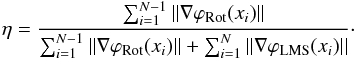 (19)This expression can be used on experimental astrophysical data.
4.3. Theoretical calculation of η
Using Eq. (19), a theoretical estimate can be made for η.
4.3.1. Estimating [[HRot]]
When observing near zenith, [[HRot]] = 0. Under these conditions, Eq. (17) can be estimated using Eq. (9). Under our stated assumption of a plane wave propagating through TAMAs followed by additional propagation, r0 does not vary with the additional propagation (see Eq. (8)). Hence, ![Mathematical equation: \begin{eqnarray} \label{eq: || H_LMS || all regimes} [[ H_{\rm LMS} ]] \propto \left\{ \begin{array}{lllll} r_0^{-5/3} & \qquad\mathrm{ for }\quad 0 < z < z_{0} \rule[-1.5ex]{0ex}{1ex} \\ r_0^{-5/3} & \qquad\mathrm{ for } \quad z_0 < z < z_{\rm ss} \rule[-1.5ex]{0ex}{1ex} \\ r_0^{-5/3} & \qquad\mathrm{ for } \quad z_{\rm ss} < z < z_{\rho_{\max}} \rule[-1.5ex]{0ex}{1ex} \\ 1/z & \qquad\mathrm{ for } \quad z_{\rho_{\max}} < z < \infty . \rule[-1.5ex]{0ex}{1ex} \\ \end{array} \right. \end{eqnarray}](/articles/aa/full_html/2013/08/aa19901-12/aa19901-12-eq123.png) (20)That is, [[HLMS]] is constant until the beam begins to diverge.
(20)That is, [[HLMS]] is constant until the beam begins to diverge.
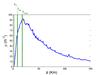 |
Fig. 4 Plot of mean branch point density versus propagation distance for r0 = 10.28 cm and averaged over twenty values of the inner scale from 0.05 to 1.0 cm. Overlaid are z0, zss and zρmax. In standard texts (Sasiela 2007), the Rytov approximation is shown to fail at |


4.3.2. Estimating [[HRot]]
Fried (1998) demonstrated that the noise-free rotational phase can be written ![Mathematical equation: \begin{eqnarray} \label{eq: BP phase} \phi_{\rm hid} = \mathrm{Im} \left\{ \sum_{k=1}^{N_{\rm BP}} h_k \log \left[ (x-x_{k}) + {\rm i}(y-y_{k}) \right] \right\} \end{eqnarray}](/articles/aa/full_html/2013/08/aa19901-12/aa19901-12-eq131.png) (21)where NBP is the number of branch points, hk is the helicity of the kth branch point, (x,y) are the coordinates, and (xk,yk) are the locations of the branch points. As a theoretical exercise, we assume that the creation pairs are known, i.e. hk and { (xi,yi) } i = 1,NBP are known. Let ⟨δ⟩ be the beam intra-pair separation for realization ℛ and
(21)where NBP is the number of branch points, hk is the helicity of the kth branch point, (x,y) are the coordinates, and (xk,yk) are the locations of the branch points. As a theoretical exercise, we assume that the creation pairs are known, i.e. hk and { (xi,yi) } i = 1,NBP are known. Let ⟨δ⟩ be the beam intra-pair separation for realization ℛ and  the phase variance of a creation pair with the mean separation, then
  (22)Note in passing that a Shack-Hartmann wavefront sensor measures
 ![Mathematical equation: \hbox{$\nabla \mathrm{Im} \left\{ \sum_{k=1}^{N_{\rm BP}} h_k \log \left[ (x-x_{k}) + {\rm i}(y-y_{k}) \right] \right\}$}](/articles/aa/full_html/2013/08/aa19901-12/aa19901-12-eq141.png) yielding for a result |∑ α ∑ khαgk| which, by Schwartz’s inequality, will underestimate the result of Eq. (22). In the case of δ ≫ Δ ≈ 10d this will greatly underestimate [[H]] because the phase averages to zero over the size of the subaperture.
yielding for a result |∑ α ∑ khαgk| which, by Schwartz’s inequality, will underestimate the result of Eq. (22). In the case of δ ≫ Δ ≈ 10d this will greatly underestimate [[H]] because the phase averages to zero over the size of the subaperture.
As a theoretical exercise, when branch points are known, Np = Aρ where A is the area of the pupil and ρ the branch point density given by Eq. (4). Combining Eqs. (18) and (22), one gets ![Mathematical equation: \begin{eqnarray} [[H_{\rm Rot}]] = \sum_\alpha \Bigl| \sum_k h_\alpha g_k \Bigr|^2 \approx N_p \sigma^2_{\rm pair} \propto \rho. \end{eqnarray}](/articles/aa/full_html/2013/08/aa19901-12/aa19901-12-eq147.png) (23)Then, by Eq. (4), to first order, [[HRot]] can be estimated as
(23)Then, by Eq. (4), to first order, [[HRot]] can be estimated as ![Mathematical equation: \begin{eqnarray} \label{eq: || H_SD || all regimes} [[ H_{\rm Rot} ]] \propto \left\{ \begin{array}{ll} 0 & \qquad\mathrm{ for }\quad 0 < z < z_{0} \rule[-1.5ex]{0ex}{1ex} \\ z^{11/6} & \qquad\mathrm{ for }\quad z_0 < z < z_{\rm ss} \rule[-1.5ex]{0ex}{1ex} \\ z^{\alpha(z)} & \qquad\mathrm{ for }\quad z_{\rm ss} < z < z_{\rho_{\max}} \rule[-1.5ex]{0ex}{1ex} \\ 1/z & \qquad\mathrm{ for } \quad z_{\rho_{\max}} < z < \infty \rule[-1.5ex]{0ex}{1ex} \\ \end{array} \right. \end{eqnarray}](/articles/aa/full_html/2013/08/aa19901-12/aa19901-12-eq149.png) (24)where α(z) bridges the gap between the unsaturated (z0 < z < zss) and saturated regimes (z > zmax).
(24)where α(z) bridges the gap between the unsaturated (z0 < z < zss) and saturated regimes (z > zmax).
4.3.3. Estimating η
Combining Eqs. (20) and (24), one obtains as a theoretical estimate of η![Mathematical equation: \begin{eqnarray} \label{eq: eta} \eta \propto \left\{ \begin{array}{lllll} 0 & \qquad\mathrm{ for } \quad 0 < z < z_{0} \rule[-1.5ex]{0ex}{1ex} \\ \rho \propto z^{11/6} & \qquad\mathrm{ for }\quad z_0 < z < z_{\rm ss} \rule[-1.5ex]{0ex}{1ex} \\ \frac{ z^{\alpha_\mathrm{max}}}{ z^{\alpha_\mathrm{max}} + r_0} < 1 & \qquad\mathrm{ for } \quad z_{\rm ss} < z < z_{\rho_{\max}} \rule[-1.5ex]{0ex}{1ex} \\ 1 & \qquad\mathrm{ for } \quad z_{\rho_{\max}} < z < \infty \rule[-1.5ex]{0ex}{1ex} \\ \end{array} \right. \end{eqnarray}](/articles/aa/full_html/2013/08/aa19901-12/aa19901-12-eq153.png) (25)where αmax is the value of α(z) at which ρBP is a maximum; experimentally, Oesch et al. (2012a) found αmax occurs at
(25)where αmax is the value of α(z) at which ρBP is a maximum; experimentally, Oesch et al. (2012a) found αmax occurs at  (see Fig. 4). Recall, this is a first order estimate which discounts saturation. On physical grounds, when saturation is accounted for, η will approach some fraction less than one; this is seen in the experimental data.
4.4. Comparison of theoretical and experimental data
The POAM fraction for atmospheric data can be calculated directly from experimental data via Eq. (19). Doing so, one can then compare Eq. (25) to experiment. [[HLMS]] and [[HRot]] are thus calculated in Fig. 5a for the data included in Fig. 3, as well as, in Fig. 5b for a wave optic simulation which uses the same turbulence parameters but over an extended propagation distance.
Figure 5a plots [[H]] over a 15 Km path for eleven values of turbulence strength as measured by r0 with each line denoting a single r0. [[HLMS]] is shown in blue. Note that for each r0, [[HLMS]] is constant, but increases with increasing r0; this is in accord with the theoretical results of Eq. (20). [[HRot]] is shown in black. Note, for all turbulence strengths, [[HRot]] is initially zero, then grows approximately quadratically until beginning to saturate at the highest values in accordance with the prediction in Eq. (24).
In Fig. 5b, [[H]] is plotted versus propagation distance for varying values of the inner scale. Similar behavior to that observed to Fig. 5a at the shortest distances, but appears to reach saturation and decrease at the highest distances.
For the data in Fig. 5, the POAM fraction is calculated using Eq. (19) and plotted in Fig. 6 with the 15 Km data on the left and 150 Km on the right. The POAM flux is zero until z0, grows quickly until an inflection point near zss, grows less quickly until saturation around η = 0.55, then remains about that value for the remainder of the propagation.
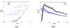 |
Fig. 5 [[H]] plotted versus propagation distance using our previously published branch point data. a) Experimental data from the 121 data sets used in Fig. 3. b) Data from wave optic simulation using the same turbulence parameters as in a). |
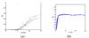 |
Fig. 6 η plotted versus propagation distance using the results in Fig. 5. a) Experimental data from the 121 data sets used in Fig. 3. b) Data from wave optic simulation using the same turbulence parameters as in a). |
4.5. Multiple TAMAs and measurement of POAM
If the atmosphere is layered or when propagating in the cosmos, the propagating wave will encounter multiple TAMAs. For multiple TAMAs or if the atmosphere is layered, to first order, the ratio of POAM to non-POAM photons is given by ![Mathematical equation: \begin{eqnarray} \label{eq: eta for multiple TAMAs} \eta = \frac{ [[ H_{\rm Rot,1} \oplus H_{\rm Rot,2} \oplus \cdots ]] } { [[ H_{\rm Rot,1} \oplus H_{\rm Rot,2} \oplus \cdots ]] + [[ H_{\rm LMS,1} \oplus H_{\rm LMS,2} \oplus \cdots ]] }\cdot \end{eqnarray}](/articles/aa/full_html/2013/08/aa19901-12/aa19901-12-eq160.png) (26)The net effect of multiple TAMAs is to increase η. Whereas in later works, it will become important to determine where POAM is created along the propagation path, in this work, it suffices to assert that astrophysical POAM exists and this is captured equally well by either Eq. (25) or Eq. (26).
(26)The net effect of multiple TAMAs is to increase η. Whereas in later works, it will become important to determine where POAM is created along the propagation path, in this work, it suffices to assert that astrophysical POAM exists and this is captured equally well by either Eq. (25) or Eq. (26).
5. On-sky measurement of POAM flux
Our previous laboratory results and theoretical considerations lead us to believe that there is an abundant supply of POAM in the galactic disk. In this section, we discuss how this flux can be measured using existing instrumentation, then present the first observations to do so.
5.1. Ideal candidate stars
The goal is to measure the POAM flux within a total photon flux of astrophysical sources. We choose to do so by observing stars. We do this for two reasons. First, properly chosen, stars are point sources, and hence the star itself contains no ϕRot. Second, stellar photon fluxes are steady although not necessarily constant.
The light from ideal candidate stars propagates through an intervening TAMA. Hence, the candidate stars, ideally, are embedded in a non-luminescent dense TAMA. Under these conditions, the physical mechanisms presented in Sects. 2−4 guarantee that POAM will be created.
T Tauri stars, with their circumstellar disks, make fine candidates. In addition, stars behind, but along the same line of sight as, proto stellar TAMAs make good candidates. For instance, O type stars, with their short lifetimes, preclude significant clearing of their local neighborhood and would appear to make good candidate stars.
These stars must also be bright, 5th magnitude or brighter for our AO system, implying that the stars reside within a few hundred parsecs of the sun.
Also, whether the star itself contains a non-zero POAM flux is irrelevant. There are indications that POAM can be created intrinsically by the sun (Uribe-Patarroyo et al. 2011) which necessarily implies this occurs in other stars, as well, and this would make the POAM flux from most stars non zero. For these observations, the mechanism of POAM creation is irrelevant, that it exists is sufficient. Obviously, later works will address the “where” more carefully.
Star list.
5.2. Data collection
The data required for calculation of η are phase gradients and these are obtained from open loop Shack-Hartmann wavefront sensor data. These gradients are the system’s calibrated gradients, i.e. the gradients found after, for instance, camera flats and gradient references, but before being fed to the AO system’s phase reconstructor (which would remove ∇ϕRot).
These gradients, being intermediate quantities in an astronomical AO system, are not typically available to the experimenter. Special consideration must be taken to ensure that they are stored to disk for later use.
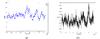 |
Fig. 7 Sample plot of the open loop data for HR 1577 taken on 2011-10-31. a) [[HLMS]] in blue and [[HRot]] in black. b) η for the data in a). Note the variability in [[HLMS]] caused by atmospheric turbulence. |
5.3. Calibration of the signal
We plan for the possibility that unknown biases exist in measurement and processing of the data. For instance, Elias (2012) demonstrates that in the radio, aberrations in the telescope can produce measurement bias of up to 10% for the Very Large Array; similar analysis has not yet been done for instrumentation in the visible, although a noise floor of 4% was found in our measurements (see Sect. 5.5.3). To account for this, we assume that any such biases are linear and can be removed through the use of reference stars. (For the record, we fully intend to identify if biases exist and remedy them in subsequent observational runs.)
Reference stars are those likely to produce a low POAM flux. The physics dictates that the reference stars share a line of sight to a candidate star, but are much closer, i.e. preferably nearby to the sun. Close proximity to the sun minimizes the chance of an intervening TAMA corrupting the reference measurement. A common line of sight ensures two things, a statistically identical sampling of Earth’s atmosphere, as well as, common instrumentation orientation of the detectors for both measurements.
In addition, the reference star is ideally a late type star, e.g. G. These stars are stable and long lived which clears their local neighborhood of their proto-stellar cloud.
5.4. Data processing
Estimation of the POAM flux can be done as presented in Sect. 4 using Eqs. (15)−(18). For each frame of wavefront sensor data, the gradients are assigned to either ℋLMS or ℋRot via  and . The estimate of HRot and HLMS for this turbulence realization is then
  where g are the measured gradients. The estimates of [[HRot]] and [[HLMS]] are then calculated using Eqs. (17) and (18).
Tabulation of [[HLMS]], [[HRot]] and η for all datasets.
5.5. Measurement of astrophysical POAM fluxes
An ad hoc set of observations to measure astrophysical POAM was proposed to our colleagues at the Starfire Optical Range and they agreed to observe, on a non-interference basis, stars from a list that we provided to them, and they, in turn, provided to us raw WFS camera frames, as well as gradients. In this way, we obtained 10 data sets for 5 stars. The purpose of these observations is merely to verify that a POAM signal exists.
The observations were conducted on the Starfire Optical Range’s 3.5 m telescope located on Kirtland AFB, NM using the natural guide star AO system with a Shack-Hartmann wavefront sensor at 450 − 650 nm with 24 × 24 subapertures and a 2 KHz open loop frame rate. The wavefront sensor resides in the coudé room.
5.5.1. The star list
Five stars were chosen. Our list includes a T-Tauri star, 49 Ceti, and another embedded in the Orion nebula, HR 1895. HR 1895 is an O type star at 490 pc, and 49 Ceti is an A type star at 61 pc. Three additional stars were chosen: HR 1529, a K type star at 72 pc, HR 1588, a K type star at 157 pc and HR 1784, a G type star at 53 pc. The star list is shown in Table 2.
With these stars we intend to establish both the system noise floor and measurement precision, then compare the stars against them.
5.5.2. Calculation of the raw POAM fluxes
For each observation, 40 000 frames of open loop wavefront sensor data were taken. For each 40 000 frame data set, a logical mask was created from the saved gradients. The mask includes points within the pupil and excludes the secondary and its struts. For each data set, a projection operator is created as detailed in Sect. 5.4. Then for each frame, HRot and HLMS are calculated via Eqs. (27) and (28). [[HRot]] and [[HLMS]] are calculated via Eqs. (17) and (18) and η is estimated using Eq. (15).
The result for a single dataset is shown pictorially in Fig. 7 for HR 1577 taken at 103941Z on 20111031. On the left, [[HRot]] and [[HLMS]] are plotted versus iteration number. Note the large fluctuations in [[HLMS]]. These are caused by atmospheric phase fluctuations. On the right, the conversion ratio for each frame calculated via Eq. (15).
The result for all data sets is tabulated in Table 3. A summary is given in Table 4.
5.5.3. Establishing the noise floor
Consider the lowest two fluxes, 0.03 and 0.04. Of the nine measurements, these occur five times. Then note the standard deviation of each is about 5 × 10⁻³.
To a few sigma, we assume with confidence that the noise floor of the system is η = 0.03 − 0.04. For the remainder of the paper, we consider it to be η = 0.04.
Mean creation efficiency for each star.
5.5.4. Evaluation of the sources
The sources can then be evaluated against the noise floor.
HR 1529 shows the highest raw flux above the noise floor. With a mean value of η = 0.07 and a standard deviation of 0.011, it lies approximately 3σ above the noise floor. 49 Ceti’s POAM flux is η = 0.06 with a standard deviation of 0.009. It lies approximately 2σ above the noise floor. HR 1577 and HR 1784 lie at the noise floor.
HR 1895 is unusual. Of the three data sets, two lie within 1σ of the noise floor, but the mean of the third, taken at 20111101 − 100929, is η = 0.17 ± 0.02, making it well above the noise floor. The cause of this large variation over a three day period is unknown, although further analysis (Oesch et al. 2013c) has shown that the 0.17 dataset is definitely signal. If the mean of the three is taken, HR 1895 has a POAM flux of 0.09, well above the noise floor. However, since the cause of this large variation over a three day period is unknown, until further examination is done, straightforward application of the mean seems questionable.
In summary, subtracting the noise floor, two of the five stars, HR 1529 and HR 1577, show POAM fluxes of η = 0.03 and η = 0.02 with certainty of 3σ and 2σ, respectively. Also, one of the three HR 1895 datasets, η = 0.17 is well above the noise floor.
5.5.5. Discussion of the on-sky data
With two of the five measurements showing signal, and an additional single data set of HR 1895 showing signal, the ad hoc experimental results indicate corroboration with theory and laboratory results. Since both theory and laboratory results definitively demonstrate that turbulence-induced POAM flux exists, we are highly encouraged that we have measured an astrophysical POAM flux. However, there remain issues for discussion.
Effect of Earth’s atmosphere on the data − 1
Earth’s atmosphere is a near TAMA which, for observations near zenith, [[HRot]] = 0 and [[HLMS]] ≠ 0. If we consider two TAMAS, Earth’s atmosphere and an astrophysical TAMA and apply Eq. (26), one obtains ![Mathematical equation: \begin{eqnarray} \label{eq: eta accounting for the near TAMA} \eta = \frac{ [[ H_{\rm Rot,star} ]] } { [[ H_{\rm Rot,star} ]] + [[ H_{\rm LMS,star} \oplus H_{\rm LMS,atmos} ]] }\cdot \end{eqnarray}](/articles/aa/full_html/2013/08/aa19901-12/aa19901-12-eq202.png) (29)The magnitude of this additional term can be large (see Fig. 7). Since the additional phase only appears in the denominator, the net effect is to lower the measured conversion ratio from the star’s actual ratio. Since non-negligible POAM fluxes were measured and the purpose here is to merely detect a POAM flux, this reduction is not a problem for these initial observations.
(29)The magnitude of this additional term can be large (see Fig. 7). Since the additional phase only appears in the denominator, the net effect is to lower the measured conversion ratio from the star’s actual ratio. Since non-negligible POAM fluxes were measured and the purpose here is to merely detect a POAM flux, this reduction is not a problem for these initial observations.
Effect of additional POAM sources on Eq. (15)
If there were multiple astrophysical TAMA, the net effect would be to increase the creation efficiency. This effect is captured in Eq. (26).
49 Ceti and HR 1895 were chosen for their proximity to known TAMAs. If another TAMA exists along the line of sight to these two stars and as a result, additional POAM flux is carried by the beam, for these first set of measurements with purpose to merely detect the POAM flux, this would be acceptable. In later observations, a means to estimate the number of and magnitude of intervening TAMA would be useful.
Effect of Earth’s atmosphere on the data − 2
Earth’s atmosphere adversely affects ground based astronomical imaging by corrupting the phase of the source beam. Since the genesis of AO (Fugate et al. 1991), the assumption of a phase-only disturbance has been shown to be remarkably good. This assumption appears implicitly through the use of Eq. (15) and is equivalent to [[HRot,atmos]] = 0. However, if the atmosphere is particularly turbulent, then the possibility exists that [[HRot,atmos]] ≠ 0.
In an attempt to explain the measurement of HR 1895 on 20111101 at 100929Z which produced η = 0.17, this must be considered. HR 1895’s altitude at this time is 47°. During the measurement, if there were particularly bad atmosphere, the inverse of Fried’s “Lucky Imaging” (Fried 1977), then perhaps Earth’s atmospheric turbulence could create hidden phase in the propagating beam causing [[HRot,atmos]] > 0. If this were true, the one “good” data set from HR 1895 could merely be noise from the atmosphere. Establishing the veracity of this possibility from our current data is not possible. But note, the data sets are 20 s in duration which would tend to mitigate a short, unlucky event. Calculation of the probability of a Fried-type “unlucky” event over twenty seconds is beyond the scope of this paper. However, this analysis does suggests that additional calibration is required in future measurements of ℋRot.
Effect of an extended object on the measurements
The Orion nebula (NGC 1976) is a bright extended object, approximately 65 arc minutes in extent with a visual magnitude of mv = 4. For a 3.5 m telescope, it is not a point source, implying ℋLMS,NGC 1976 ≠ 0. Since HR 1895 is embedded in NGC 1976, measurements of it will contain gradients from the nebula. The net effect is captured in Eq. (29) as when considering Earth’s atmosphere, and this is to lower the measured conversion ratio from the star’s actual ratio, i.e. the denominator of Eq. (15) would go to [[HRot + HLMS + HLMS,NGC 1976]]. Again, since non-negligible POAM fluxes were measured, this reduction is not a problem for these initial observations. This, however, should be accounted for in future observations, but does not alter our stated results.
The Shack-Hartman wavefront sensor gain curve and its impact on our measurements
Shack-Hartman wavefront sensors estimate gradients non-linearly, so that for small tilts, the estimation of the gradient is quite good, but for large tilts, the estimation saturates to a constant value. This gives Shack-Hartman wavefront sensors a high dynamic range which is ideal for imaging, but for our measurements here, this means that calculation of [[HLMS]] and [[HRot]] will saturate, as well.
For the data presented here, there is no means to determine the extent of the saturation. However, in future experiments, this issue must be corrected, and can easily be done through, for instance, the use of a higher density wavefront sensor. Doing so, of course, will be at the expense of reduced sky coverage.
The effects of instrumentation on the measurement
Elias (2008, 2012) demonstrated that instrumentation affects the measurement of POAM and notes that polarization (spin angular momentum) can be measured as orbital angular momentum. The degree to which this occurs can depend on the azimuth and elevation of the telescope, as well as, the optics leading to the detector. For this first set of measurements, we assume that a proper choice of reference stars addresses this issue. This assumption bears close scrutiny. Our analysis in Sects. 5.5.2–5.5.4 merely established a noise floor of the device without regard to lines of sight. Considering lines of sight, the nearest reference star is approximately within 10o of a candidate. Whether this is acceptable will only be known with further analysis, and this analysis must be a prerequisite for follow-on observations.
It bears study whether the converse is also true, i.e. that POAM will be measured as polarization. The result of this analysis can have interesting repercussions, namely that POAM has been measured for some time by astronomical instruments, but attributed incorrectly.
Chromaticity and measurement of ℋRot
The effect of a broad spectrum is to smear the gradients in ℋRot making them appear near zero. This will cause the measured value of [[HRot]] to be underestimated with respect to its actual value, but, again, as long as [[HRot]] is above the noise floor, this is not a problem. Filters can be used to address this problem, but doing so would further restrict the number of candidate stars.
The effect of Δ and δ on data collection
In the astrophysical regime, Δ and δ are much larger than those found in laboratory data. Classic AO wavefront sensor’s subaperture spacing is tied to Fried’s parameter. Hence, δ ≫ Δ ≫ d, so, existing wavefront sensors will measure averaged values ϕRot. As was discussed in Sect. 4.3.2, this causes an underestimation of ϕRot. Additionally, since d ≪ Δ, this precludes the use of Eq. (3) in identifying branch points. The full implication of these statements are not yet clear, although over the long term, the solution will be to create direct OAM detectors tailored for measurement of astrophysical POAM.
5.6. Summary of the on-sky data
The purposes of this section were to enumerate a means to measure the astrophysical POAM flux and to present the results of ad hoc observations. The former is enumerated in Sects. 5.1−5.4, and the latter accomplished in Sect. 5.5. Using those techniques, a POAM flux of 2 − 3% of the total photon flux with confidence of 2 − 3σ. We consider this to be tentative observational detection of our theoretical predictions, which are based on our previous results.
6. Conclusions
Theory, simulation, laboratory, and now on-sky measurements support the thesis that a significant number of astrophysical POAM photons exist. We are led by our previous laboratory data to conclude that under the right circumstances, the POAM flux will reach approximately half of the total photon flux but for the on-sky data presented here, it was found to be as large as 17% of the total photon flux. Since the conditions for POAM creation are so ubiquitous, we expect to find POAM fluxes existing in varying strengths throughout the cosmos.
Online material
Appendix A: The projection operators – A history of POAM in adaptive optics
Fugate et al. (1991) created AO, and in doing so, demonstrated a means to compensate for atmospheric turbulence through the use of a wavefront sensor and a deformable mirror. The wavefront sensor measures phase and, through processing, returns the deformable mirror commands that compensate for the phase disturbance. Since the measurement contains noise, in order to ensure optimal performance, the measurements must be filtered; in AO, this process is called reconstruction of the phase, and the matrix that does the reconstruction is called the reconstructor.
In retrospect, the AO reconstructor is the keystone that allowed for creating the projection operator onto ℋRot. Sections A.1–A.5 illuminate how this is so.
Appendix A.1: Minimization of noise – The first reconstructor
Following Fugate (2001), assume the sensor is a Shack-Hartmann wavefront sensor; this sensor discretizes the field and returns phase gradients. Let each discretely measured element be called a subaperture. For each subaperture, we wish to estimate the deformable mirror command required to correct the phase aberration in that subaperture. In this light, let a be the deformable mirror actuator commands for all subapertures (i.e. the optical path difference (OPD) required to remove phase in each subaperture), and let g be the phase gradients for all subapertures.
Adaptive optics fundamentally assumes that the atmosphere is a smooth disturbance that exists in the pupil of the telescope, and further that the AO system is optically conjugate to the turbulence. Under these assumptions (and no noise), g is continuous and  (A.1)where Γ is a matrix that converts actuator commands (i.e. phase) into phase gradients. We need to solve for the deformable mirror commands, a, given the measurements g, and this must be done in the presence of noise. (Note that under the stated assumptions, the discontinuous part of g is considered noise.)
Letting â be the actuator commands in the presence of noise, the minimum error solution in the least mean square sense is given by the minimization of |g − Γâ|. The solution is given by  (A.2)where Γ† is the pseudo inverse. The left hand side of Eq. (A.2) is the AO compensation which returns the optimal phase for imaging.
Equation (A.2) is the reconstruction process and Γ† is the AO reconstructor.
Appendix A.2: Branch points in AO
Fried (1998) when studying the branch point problem in AO, considered both the gradients associated with â, as well as, the remainder of the gradients. In doing so, he illustrated that the total phase, ϕ is uniquely comprised of two phases, ϕLMS and ϕRot, with ϕRot caused by branch points, and further that the gradients of these phases, ∇ϕLMS and ∇ϕRot, are orthogonal i.e. ϕ = ϕLMS + ϕRot with  In the terms of the previous subsection,
  ; also, the gradients ∇ϕRot are considered noise by the reconstructor, and hence, are rejected. This fact led Fried (1998) in his seminal paper to call ϕRot the “hidden phase”.
In the evolution of theory, the phase which was originally viewed as a least mean square solution to a noise problem, ϕLMS, now also defines another phase, ϕRot, which is due to branch points. At this point in conventional wisdom, since branch points were seen to randomly appear and disappear in all experimental data, they were still considered a noise problem.
Appendix A.3: Branch points as enduring features of the traveling wave
Sanchez & Oesch (2009) and Oesch et al. (2010) later demonstrated that a component of ϕRot was not noise at all, but an enduring feature of the traveling wave. That branch points seemingly randomly appeared and disappeared in experimental data was shown to be a measurement problem. Note for clarity, in experimental data, both ϕLMS and ϕRot contain noise, and while noise must be dealt with when analyzing data, it is not our concern here.
At this point in the evolution of theory, both ϕLMS and ϕRot are physical features of the traveling wave, caused directly and indirectly by turbulence, respectively.
Appendix A.4: The two orthogonal Hilbert spaces and the projection operators
Consider the gradients gâ such that 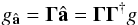 (A.5)The operator ΓΓ† is a projection of the total gradients, g, onto gâ. Denote the remainder of the gradients
  . Then,
  (A.6)where is the identity operator. is a projection operator of g onto . Brennan (2007 priv. comm. TR-1648) demonstrated that the gradients gâ and define two orthogonal Hilbert spaces, ℋLMS and ℋRot, such that ℋ = ℋLMS ⊕ ℋRot, and he derived a sparse basis for ℋRot. In this light, ΓΓ† is a projection operator (called earlier in the text) that selects the gradients in ℋLMS. Similarly, is a projection operator onto ℋRot. Note, since SH WFSs discretize the phase, and are matrices.
In the notation of Fried (1998) and writing the phase in units of OPD, the gradients  due to branch points define a Hilbert space ℋRot. Since the gradients are random variables, knowing that the gradients lie in Hilbert spaces, gives a ready means, through the norm of the Hilbert space, to estimate their size.
At this point in the evolution of theory, a means was in hand to estimate the relative quantity of the stochastically generated non-zero elements in ℋLMS and ℋRot (this was presented as the ratio η earlier in the text).
Appendix A.5: POAM in the traveling wave
To complete the history, Sanchez & Oesch (2011a,b) later established that ![Mathematical equation: \hbox{$[[ \bfg_\bfbhat ]] \ne 0$}](/articles/aa/full_html/2013/08/aa19901-12/aa19901-12-eq238.png) implies that the traveling wave is carrying non-zero POAM, and realized a short time later, it would be possible to show that a good fraction, perhaps most, of the photons in the universe carry non-zero POAM.
implies that the traveling wave is carrying non-zero POAM, and realized a short time later, it would be possible to show that a good fraction, perhaps most, of the photons in the universe carry non-zero POAM.
Appendix B: Plots of the on sky data
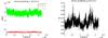 |
Fig. B.1 49 Ceti. Left column: [[H]]. Right column: η. |
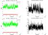 |
Fig. B.2 HR 1529. Left column: [[H]]. Right column: η. |
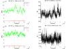 |
Fig. B.3 HR 1577. Left column: [[H]]. Right column: η. |
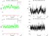 |
Fig. B.4 HR 1784. Left column: [[H]]. Right column: η. |
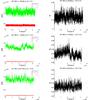 |
Fig. B.5 HR 1895. Left column: [[H]]. Right column: η. |
Acknowledgments
We extend our appreciation to Dr. Terry Brennan who graciously allowed us to use his techniques for obtaining and further insisted that no distinctive citation within the text was necessary. Additionally, we extend special thanks to Dr. Nicholas Elias whose insightful comments greatly improved this paper.
References
- Allen, L., Beijersbergen, M. W., Spreeuw, R. J. C., & Woerdman, J. P. 1992,Phys. Rev. A, 45, 8185 [Google Scholar]
- Andrews, L. C., & Phillips, R. L. 1998, Laser Beam Propagation through Random Media, 2nd edn. (Bellingham, WA, USA: SPIE Press) [Google Scholar]
- Berkhout, G. C. G., & Beijersbergen, M. W. 2009, J. Opt. A, 11, 094021 [NASA ADS] [CrossRef] [Google Scholar]
- Berkhout, G. C. G., & Beijersbergen, M. W. 2010, Phys. Rev. Lett., 101, 100801 [Google Scholar]
- Berkhout, G. C. G., Lavery, M. P. J., Padgett, M. J., & Beijersbergen, M. W. 2011, Opt. Lett., 36, 1863 [NASA ADS] [CrossRef] [Google Scholar]
- Brennan, T. J., & Mann, D. C. 2010, Proc. SPIE, 7816, 781602 [CrossRef] [Google Scholar]
- Chen, X.-S., Lü, X.-F., Sun, W.-M., Wang, F., & Goldman, T. 2008, Phys. Rev. Lett., 100, 232002 [NASA ADS] [CrossRef] [PubMed] [Google Scholar]
- Elias, II, N. M. 2008, A&A, 492, 883 [NASA ADS] [CrossRef] [EDP Sciences] [Google Scholar]
- Elias, II, N. M. 2012, A&A, 541, A1 [Google Scholar]
- Farrell, T. C., Sanchez, D. J., Smith, J. C., et al. 2012, Proc. SPIE, 8520, 85200 [CrossRef] [Google Scholar]
- Fried, D. L. 1977,J. Opt. Soc. Am. , 40, 1651 [Google Scholar]
- Fried, D. L. 1998,J. Opt. Soc. Am. A, 15, 2759 [Google Scholar]
- Fried, D. L., & Vaughn, J. L. 1992, Appl. Opt., 31, 2865 [NASA ADS] [CrossRef] [Google Scholar]
- Fugate, R. Q. 2001, Adaptive Optics, 2nd edn., eds. M. Bass, J. M. Enoch, E. W. Van Stryland, & W. L. Wolfe (New York: USA: McGraw-Hill), Handbook of Optics, 3, 1.3 [Google Scholar]
- Fugate, R. Q., et al. 1991, Nature, 353, 144 [NASA ADS] [CrossRef] [Google Scholar]
- Gikhman, I. I., & Skorokhod, A. V. 1969, Introduction to the Theory of Random Processes, 1st edn. (Mineola, New York, USA: Dover Publications, Inc.) (an English translation of the original work) [Google Scholar]
- Harwit, M. 2003, ApJ, 597, 1266 [NASA ADS] [CrossRef] [Google Scholar]
- Hemsing, E., Knyazik, A., O’Shea, F., et al. 2012, Appl. Phys. Lett., 100, 901110 [CrossRef] [Google Scholar]
- Hill, R. J., & Ochs, G. R. 1992,J. Opt. Soc. Am. A, 9, 1406 [Google Scholar]
- Jackson, J. D. 1975, Classical Electrodynamics, 2nd edn. (New York, USA: John Wiley & Sons) [Google Scholar]
- Lavery, M. P. J., Berkhout, G. C. G., Courtial, J., & Padgett, M. J. 2011, J. Opt., 13, 064006 [NASA ADS] [CrossRef] [Google Scholar]
- Leach, J., Keen, S., Padgett, M. J., Saunter, C., & Love, G. D. 2006,Opt. Express, 14, 11919 [Google Scholar]
- Mohammadi, S. M., Daldorff, L. K. S., Forozesh, K., & Thidé, B. 2010, Rad. Sc., 45, RS4007 [Google Scholar]
- Murphy, K., Burke, D., Devaney, N., & Dainty, C. 2010,Opt. Express, 18, 15448 [Google Scholar]
- Oesch, D. W., & Sanchez, D. J. 2012,Opt. Express, 20, 12292 [Google Scholar]
- Oesch, D. W., Sanchez, D. J., & Matson, C. L. 2010,Opt. Express, 18, 22377 [Google Scholar]
- Oesch, D. W., Sanchez, D. J., & Kelly, P. R. 2012a, OSA Technical Digest (online), FW3A.3 [Google Scholar]
- Oesch, D. W., Sanchez, D. J., & Kelly, P. R. 2012b, OSA Technical Digest (online), FW2D.3 [Google Scholar]
- Oesch, D. W., Sanchez, D. J., & Tewksbury-Christle, C. M. 2012c,Opt. Express, 2, 1046 [Google Scholar]
- Oesch, D. W., Tewksbury-Christle, C. M., Sanchez, D. J., & Kelly, P. R. 2012d, Opt. Eng. , 51, 106001 [NASA ADS] [CrossRef] [Google Scholar]
- Oesch, D. W., Sanchez, D. J., Gallegos, A. L., et al. 2013a,Opt. Express, 21, 5440 [Google Scholar]
- Oesch, D. W., Sanchez, D. J., Gallegos, A. L., et al. 2013b, in Propagation through and Characterization of Distributed Volume Turbulence (Optical Society of America), submitted [Google Scholar]
- Oesch, D. W., Sanchez, D. J., & Kelly, P. R. 2013c, in Propagation through and Characterization of Distributed Volume Turbulence (Optical Society of America), submitted [Google Scholar]
- Parkin, S., Knoner, G., Nieminen, T. A., Heckenberg, N. R., & Rubinsztein-Dunlop, H. 2006,Opt. Express, 14, 6963 [Google Scholar]
- Peele, A. G., McMahon, P. J., Paterson, D., et al. 2002, Opt. Lett., 20, 1752 [NASA ADS] [CrossRef] [Google Scholar]
- Sanchez, D. J., & Oesch, D. W. 2009, Proc. SPIE, 7466, 0501 [Google Scholar]
- Sanchez, D. J., & Oesch, D. W. 2011a,Opt. Express, 19, 25388 [Google Scholar]
- Sanchez, D. J., & Oesch, D. W. 2011b,Opt. Express, 19, 24596 [Google Scholar]
- Sanchez, D. J., & Oesch, D. W. 2012, Proc. SPIE, 8520, 852004 [CrossRef] [Google Scholar]
- Sanchez, D. J., Oesch, D. W., & Kelly, P. R. 2010, Proc. SPIE, 7816, 0701 [Google Scholar]
- Sanchez, D. J., Oesch, D. W., & Kelly, P. R. 2012, Proc. SPIE, 8380, 83800P [Google Scholar]
- Sasiela, R. J. 2007, Electromagnetic Wave Propagation in Turbulence: Evaluation and Application of Mellin Transforms, 2nd edn. (Bellingham, Wa, USA: SPIE Press) [Google Scholar]
- Tamburini, F., Thidé, B., Molina-Terriza, G., & Anzolon, G. 2011, Nat. Phys. Lett. , 7, 195 [CrossRef] [Google Scholar]
- Tao, D., Wen-Feng, L., & Xiao-Hua, W. 2011, Comm. Th. Phys. , 55, 1041 [CrossRef] [Google Scholar]
- Uribe-Patarroyo, N., Alvarez-Herrero, A., Ariste, A. L., et al. 2011, A&A, 526, A56 [NASA ADS] [CrossRef] [EDP Sciences] [Google Scholar]
All Tables
All Figures
|
Fig. 1 a) Phase of a single branch point, if it could exist in nature. Also, the phase for the m = 1 Laguerre-Gaussian beam which is known to rapidly decohere in the presence of turbulence. b) ϕRot for a distribution of creation pairs with an overlay of Δ and δ. The scale on both plots is [− π,π]. |
| In the text | |
|
Fig. 2 Experimental data of ϕRot, a) low branch point density, b) high branch point density. The scale on both plots is [− π,π]. |
| In the text | |
|
Fig. 3 ASALT laboratory data highlighting creation pair behavior. Eleven values of turbulence strength with r0 in the range 6.5 − 16.6 cm. a) Intra-pair separation as a function of normalized distance. b) The inverse of the inter-pair separation, i.e. branch point density, as a function of propagation distance. |
| In the text | |
|
Fig. 4 Plot of mean branch point density versus propagation distance for r0 = 10.28 cm and averaged over twenty values of the inner scale from 0.05 to 1.0 cm. Overlaid are z0, zss and zρmax. In standard texts (Sasiela 2007), the Rytov approximation is shown to fail at |
| In the text | |
|
Fig. 5 [[H]] plotted versus propagation distance using our previously published branch point data. a) Experimental data from the 121 data sets used in Fig. 3. b) Data from wave optic simulation using the same turbulence parameters as in a). |
| In the text | |
|
Fig. 6 η plotted versus propagation distance using the results in Fig. 5. a) Experimental data from the 121 data sets used in Fig. 3. b) Data from wave optic simulation using the same turbulence parameters as in a). |
| In the text | |
|
Fig. 7 Sample plot of the open loop data for HR 1577 taken on 2011-10-31. a) [[HLMS]] in blue and [[HRot]] in black. b) η for the data in a). Note the variability in [[HLMS]] caused by atmospheric turbulence. |
| In the text | |
|
Fig. B.1 49 Ceti. Left column: [[H]]. Right column: η. |
| In the text | |
|
Fig. B.2 HR 1529. Left column: [[H]]. Right column: η. |
| In the text | |
|
Fig. B.3 HR 1577. Left column: [[H]]. Right column: η. |
| In the text | |
|
Fig. B.4 HR 1784. Left column: [[H]]. Right column: η. |
| In the text | |
|
Fig. B.5 HR 1895. Left column: [[H]]. Right column: η. |
| In the text | |
Current usage metrics show cumulative count of Article Views (full-text article views including HTML views, PDF and ePub downloads, according to the available data) and Abstracts Views on Vision4Press platform.
Data correspond to usage on the plateform after 2015. The current usage metrics is available 48-96 hours after online publication and is updated daily on week days.
Initial download of the metrics may take a while.