| Issue |
A&A
Volume 556, August 2013
|
|
|---|---|---|
| Article Number | A130 | |
| Number of page(s) | 13 | |
| Section | Astrophysical processes | |
| DOI | https://doi.org/10.1051/0004-6361/201219901 | |
| Published online | 05 September 2013 | |
Online material
Appendix A: The projection operators – A history of POAM in adaptive optics
Fugate et al. (1991) created AO, and in doing so, demonstrated a means to compensate for atmospheric turbulence through the use of a wavefront sensor and a deformable mirror. The wavefront sensor measures phase and, through processing, returns the deformable mirror commands that compensate for the phase disturbance. Since the measurement contains noise, in order to ensure optimal performance, the measurements must be filtered; in AO, this process is called reconstruction of the phase, and the matrix that does the reconstruction is called the reconstructor.
In retrospect, the AO reconstructor is the keystone that allowed for creating the projection operator onto ℋRot. Sections A.1–A.5 illuminate how this is so.
Appendix A.1: Minimization of noise – The first reconstructor
Following Fugate (2001), assume the sensor is a Shack-Hartmann wavefront sensor; this sensor discretizes the field and returns phase gradients. Let each discretely measured element be called a subaperture. For each subaperture, we wish to estimate the deformable mirror command required to correct the phase aberration in that subaperture. In this light, let a be the deformable mirror actuator commands for all subapertures (i.e. the optical path difference (OPD) required to remove phase in each subaperture), and let g be the phase gradients for all subapertures.
Adaptive optics fundamentally assumes that the atmosphere is a smooth disturbance that exists in the pupil of the telescope, and further that the AO system is optically conjugate to the turbulence. Under these assumptions (and no noise), g is continuous and  (A.1)where Γ is a matrix that converts actuator commands (i.e. phase) into phase gradients. We need to solve for the deformable mirror commands, a, given the measurements g, and this must be done in the presence of noise. (Note that under the stated assumptions, the discontinuous part of g is considered noise.)
Letting â be the actuator commands in the presence of noise, the minimum error solution in the least mean square sense is given by the minimization of |g − Γâ|. The solution is given by  (A.2)where Γ† is the pseudo inverse. The left hand side of Eq. (A.2) is the AO compensation which returns the optimal phase for imaging.
Equation (A.2) is the reconstruction process and Γ† is the AO reconstructor.
Appendix A.2: Branch points in AO
Fried (1998) when studying the branch point problem in AO, considered both the gradients associated with â, as well as, the remainder of the gradients. In doing so, he illustrated that the total phase, ϕ is uniquely comprised of two phases, ϕLMS and ϕRot, with ϕRot caused by branch points, and further that the gradients of these phases, ∇ϕLMS and ∇ϕRot, are orthogonal i.e. ϕ = ϕLMS + ϕRot with  In the terms of the previous subsection,
  ; also, the gradients ∇ϕRot are considered noise by the reconstructor, and hence, are rejected. This fact led Fried (1998) in his seminal paper to call ϕRot the “hidden phase”.
In the evolution of theory, the phase which was originally viewed as a least mean square solution to a noise problem, ϕLMS, now also defines another phase, ϕRot, which is due to branch points. At this point in conventional wisdom, since branch points were seen to randomly appear and disappear in all experimental data, they were still considered a noise problem.
Appendix A.3: Branch points as enduring features of the traveling wave
Sanchez & Oesch (2009) and Oesch et al. (2010) later demonstrated that a component of ϕRot was not noise at all, but an enduring feature of the traveling wave. That branch points seemingly randomly appeared and disappeared in experimental data was shown to be a measurement problem. Note for clarity, in experimental data, both ϕLMS and ϕRot contain noise, and while noise must be dealt with when analyzing data, it is not our concern here.
At this point in the evolution of theory, both ϕLMS and ϕRot are physical features of the traveling wave, caused directly and indirectly by turbulence, respectively.
Appendix A.4: The two orthogonal Hilbert spaces and the projection operators
Consider the gradients gâ such that 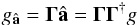 (A.5)The operator ΓΓ† is a projection of the total gradients, g, onto gâ. Denote the remainder of the gradients
  . Then,
 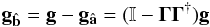 (A.6)where is the identity operator. is a projection operator of g onto . Brennan (2007 priv. comm. TR-1648) demonstrated that the gradients gâ and define two orthogonal Hilbert spaces, ℋLMS and ℋRot, such that ℋ = ℋLMS ⊕ ℋRot, and he derived a sparse basis for ℋRot. In this light, ΓΓ† is a projection operator (called
  earlier in the text) that selects the gradients in ℋLMS. Similarly, is a projection operator onto ℋRot. Note, since SH WFSs discretize the phase, and
  are matrices.
In the notation of Fried (1998) and writing the phase in units of OPD, the gradients  due to branch points define a Hilbert space ℋRot. Since the gradients are random variables, knowing that the gradients lie in Hilbert spaces, gives a ready means, through the norm of the Hilbert space, to estimate their size.
At this point in the evolution of theory, a means was in hand to estimate the relative quantity of the stochastically generated non-zero elements in ℋLMS and ℋRot (this was presented as the ratio η earlier in the text).
Appendix A.5: POAM in the traveling wave
To complete the history, Sanchez & Oesch (2011a,b) later established that  implies that the traveling wave is carrying non-zero POAM, and realized a short time later, it would be possible to show that a good fraction, perhaps most, of the photons in the universe carry non-zero POAM.
Appendix B: Plots of the on sky data
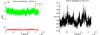 |
Fig. B.1
49 Ceti. Left column: [[H]]. Right column: η. |
| Open with DEXTER | |
 |
Fig. B.2
HR 1529. Left column: [[H]]. Right column: η. |
| Open with DEXTER | |
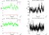 |
Fig. B.3
HR 1577. Left column: [[H]]. Right column: η. |
| Open with DEXTER | |
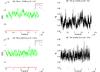 |
Fig. B.4
HR 1784. Left column: [[H]]. Right column: η. |
| Open with DEXTER | |
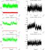 |
Fig. B.5
HR 1895. Left column: [[H]]. Right column: η. |
| Open with DEXTER | |
© ESO, 2013
Current usage metrics show cumulative count of Article Views (full-text article views including HTML views, PDF and ePub downloads, according to the available data) and Abstracts Views on Vision4Press platform.
Data correspond to usage on the plateform after 2015. The current usage metrics is available 48-96 hours after online publication and is updated daily on week days.
Initial download of the metrics may take a while.