| Issue |
A&A
Volume 525, January 2011
|
|
|---|---|---|
| Article Number | A38 | |
| Number of page(s) | 8 | |
| Section | Extragalactic astronomy | |
| DOI | https://doi.org/10.1051/0004-6361/201015575 | |
| Published online | 30 November 2010 | |
Suzaku and SWIFT-BAT observations of a newly discovered Compton-thick AGN
1
INAF - Osservatorio Astronomico di Brera, via Brera 28, 20121
Milano, Italy
e-mail: paola.severgnini@brera.inaf.it
2
Department of Physics and Astronomy, Leicester
University, Leicester, LE1
7RH, UK
3
Dipartimento di Astronomia, Universita’ degli Studi di
Bologna, via Ranzani
1, 40127
Bologna,
Italy
4
INAF – Osservatorio Astronomico di Bologna,
via Ranzani 1, 40127
Bologna,
Italy
5
INAF – Istituto di Astrofisica Spaziale e Fisica Cosmica di
Palermo, via U. La Malfa
153, 90146
Palermo,
Italy
Received: 12 August 2010
Accepted: 6 October 2010
Context. Obscured AGN are fundamental to understand the history of supermassive black hole growth and their influence on galaxy formation. However, the Compton-thick AGN (NH > 1024 cm-2) population is basically unconstrained, with less than a few dozen confirmed Compton-thick AGN found and studied so far. A way to select heavily obscured AGN is to compare the X-ray emission below 10 keV (which is strongly depressed) with the emission from other bands that are less affected by the absorption, like the IR band. To this end, we have cross-correlated the 2XMM catalogue with the IRAS Point Source catalogue and, by using the X-ray to infrared flux ratio and X-ray colours, we selected a well defined sample of Compton-thick AGN candidates at z < 0.1.
Aims. The aim of this work is to confirm the nature and to study one of these local Compton-thick AGN candidates, the nearby (z = 0.029) Seyfert 2 galaxy IRAS 04507+0358, by constraining the amount of intrinsic absorption (NH) and thus the intrinsic luminosity.
Methods. To this end we obtained deep (100 ks) Suzaku observations (AO4 call) and performed a joint fit with SWIFT-BAT data. We analysed XMM-Newton, Suzaku and SWIFT-BAT data and present here the results of this broad-band (0.4−100 keV) spectral analysis.
Results. We found that the broad-band X-ray emission of IRAS 04507+0358 requires a large amount of absorption (higher than 1024 cm-2) to be well reproduced, thus confirming the Compton-thick nature of this source. In particular, the most probable scenario is that of a mildly (NH ~ 1.3−1.5 × 1024 cm-2, L(2−10 keV) ~ 5−7 × 1043 erg s-1) Compton-thick AGN.
Key words: galaxies: active / galaxies: individual: IRAS 04507+0358 / galaxies: Seyfert / X-rays: galaxies
© ESO, 2010
1. Introduction
On the basis of the most accredited X-ray background synthesis models (Gilli et al. 1997; Treister et al. 2009; Ballantyne et al. 2006), obscured AGN (NH > 1022 cm-2) dominate the entire AGN population. For this reason, their space density at different redshifts is one of the main ingredients in setting the evolutionary properties of the supermassive black hole (SMBH). Unfortunately, the absorption of the obscuring medium (composed of gas and dust) along the line of sight does not allow us to easily detect them and study their nuclear properties in the UV/optical bands and in the soft X-ray bands (energy below few keV). This is particularly true for the most obscured sources, the so called Compton-thick AGN, which are hidden by a large amount of circum-nuclear obscuring matter along the line of sight (column density of NH > 1024 cm-2).
Compton-thick AGN are generally divided into two main classes of sources: mildly Compton-thick with NH of the order of a few times 1024 cm-2 and heavily Compton-thick with NH above ~1025 cm-2. The primary radiation is strongly suppressed at low energies for mildly Compton-thick AGN, emerging only above 10 keV, while for heavily Compton-thick AGN the primary radiation is strongly depressed above 10 keV as well, because of the compton down-scattering effect (Matt 1996). In both classes of sources, the spectrum below 10 keV is dominated by a pure reflection component (i.e. the continuum emission reflected by the putative torus), which is much fainter than the direct one. For this reason, even for intrinsically luminous objects, it is generally difficult to accumulate enough counts below 10 keV to allow us a reliable spectral analysis and thus to assess the nature of these sources. Furthermore, even when the spectral analysis is possible, the absorption cut-off is only marginally detectable below 10 keV (or completely outside the observed energy window). This does not allow us to correctly measure the intrinsic absorption and therefore to estimate the nuclear luminosity. Moreover, as we will show in this paper, in spite of the different values of intrinsic NH, the shape of Compton-thin AGN with 5 × 1023 cm-2 < NH < 1024 cm-2 and Compton-thick AGN spectra below 10 keV may appear very similar and indistinguishable, especially in cases of low counting statistics. This makes it even more difficult to adequately probe the heavily obscured AGN population. Often the presence of Compton thick matter is inferred through indirect arguments, such as the presence of a strong iron emission line at 6.4 keV; for high values of NH, the equivalent width of this line is expected to be high, reaching values as a few keV (Matt et al. 1996; Murphy & Yaqoob 2009).
To properly set the presence of a Compton-thick source and measure the amount of absorption, hard X-ray data above 10 keV are needed (Comastri et al. 2010). These data allow us to detect the absorption cut-off in the very hard X-ray domain typical of the large amount of intrinsic NH (>1024 cm-2). For the vast majority of Compton-thick AGN without high-energy data, we can give only a conservative lower limit on the intrinsic column density and nuclear luminosity. Extreme examples of these limitations are NGC 6240 (Vignati et al. 1999), Mrk 231 (Braito et al. 2004) and Arp 299 (Della Ceca et al. 2002), where only Beppo-SAX PDS (energy range 15 − 300 keV) observations were able to reveal the intrinsic AGN emission, allowing the direct measure of the NH and the intrinsic AGN luminosity.
A reliable estimate of the number of Compton-thick AGN requires first of all the use of efficient methods able to select large and possibly complete samples of Compton-thick AGN candidates. As a second step, broad-band X-ray spectra (from a few to hundreds keV) are needed to confirm their Compton-thick nature. However, we lack such a statistical sample and, more importantly, only a limited fraction of the putative Compton thick AGN have been confirmed through broad-band X-ray spectroscopy (see Comastri et al. 2004; Della Ceca et al. 2008a; Awaki et al. 2000; Teng et al. 2009; Braito et al. 2009). For this reason, indirect arguments are generally used to estimate their density in the local Universe (Della Ceca et al. 2008b).
In Severgnini et al. (2010) we found that the (2 − 10 keV) to 24 μm flux ratio vs. X-ray colours can be used as an efficient technique to select Compton-thick candidates, at least in the local Universe. In particular, after cross-correlating the IRAS Point Source Catalog v2.1 (PSC) with the bright end (F2 − 10 keV > 10-13 erg cm-2 s-1) of the incremental version of the 2XMM catalogue (Watson et al. 2009), we found that 85% of the 46 extragalactic sources with F(2 − 10 keV)/(ν24 μmF24 μm) < 0.03 and HR41 > −0.1 have X-ray properties resembling those of a typical Compton-thick AGN. Ten of these are newly discovered Compton-thick candidates. In order to confirm the nature of these objects, we both cross-correlated our Compton-thick AGN candidates with the SWIFT-BAT catalogue (54 months of observations, Cusumano et al. 2010) and obtained Suzaku observations for two of them (IRAS 04507+0358 and MCG-03-58-007). Here we present the results obtained with the broad-band X-ray analysis (Suzaku plus SWIFT-BAT) of IRAS 04507+0358, the first target observed by Suzaku, while the results obtained with the cross-correlation with the SWIFT-BAT catalogue will be presented in a forthcoming paper (Severgnini et al., in prep.). Throughout this paper we use the cosmological parameters H0 = 71 km s-1 Mpc-1, Ωλ = 0.7 and ΩM = 0.3.
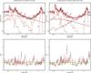 |
Fig. 1 XMM-Newton (MOS1 – black data points in the electronic version and MOS2 – red data points in the electronic version) unfolded spectrum of IRAS 04507+0358 fitted with a Compton-thin (left panel) and a Compton-thick model (right panel). In the lower panels the ratio between data and best-fit models are shown. In the Compton-thin hypothesis, the data are best reproduced by two thermal emission components (a), b)) plus a power-law absorbed only by the Galactic column density (scattering component, c)) and a power-law absorbed by a high column density (NH = (4 ± 2) × 1023 cm-2) absorber e). The two power-laws have the same Γ fixed to 1.9. A prominent iron line is also present d). A similarly good fit could be obtained by using a cold reflection component instead of the absorbed power-law (component e) in the right panel). |
2. IRAS 04507+0358
This source is optically classified as a Seyfert 2 galaxy at z = 0.029 (Strauss et al. 1992). No clear signs of starburst activity have been detected (Cid Fernandes et al. 2001). From the IRAS-PSC catalogue fluxes we calculated the infrared (8 − 1000 μm) luminosity following the prescription reported in Sanders & Mirabel (1996) and Risaliti et al. (2000). We found LIR ≃ 2.7 × 1044 erg s-1 ≃ 7 × 10¹⁰ L⊙, in agreement with the estimate reported in Fraquelli et al. (2003).
2.1. XMM-Newton archival data
The 2–10 keV spectrum used in the analysis described here (Observation ID = 0307000401,
~ 11 ks of good time exposure in the MOS camera only) was taken from the
XMM-Newton archive as one of the products of the 2XMM catalogue (Watson
et al. 2009). The data are grouped with a minimum
of 20 counts per channel. The X-ray emission of IRAS 04507+0358
(F(2−10 keV) ~
10-12 erg cm-2 s-1) could be explained with two formally
acceptable models: a transmission dominated (NH <
1024 cm-2) and a reflection (NH ≫
1024 cm-2) dominated scenario (see Fig. 1). In both cases, two thermal components are required to fit the softer
part of the spectrum (below 2 keV). We used two mekal models (Mewe et al.
1985, 1986; Liedahl et al. 1995) with the
abundances of Wilms et al. (2000), which are
typical of the inter-stellar medium. We found kT1 =
0.15 and kT2 =
0.72
and kT2 =
0.72 keV (if we use the Compton-thin model) and
kT2 = 0.66
keV (if we use the Compton-thin model) and
kT2 = 0.66 keV (if we use the Compton-thick model).
These thermal components are most probably associated to star-forming activity. As we will
discuss in Sect. 3, we estimated a star-formation rate (SFR) of about
10 M⊙/yr in our source on the basis of the infrared
luminosity. For these values of SFR, multi-temperature components in the X-ray spectra are
generally observed (e.g. M 82, Persic et al. 2004).
keV (if we use the Compton-thick model).
These thermal components are most probably associated to star-forming activity. As we will
discuss in Sect. 3, we estimated a star-formation rate (SFR) of about
10 M⊙/yr in our source on the basis of the infrared
luminosity. For these values of SFR, multi-temperature components in the X-ray spectra are
generally observed (e.g. M 82, Persic et al. 2004).
As for the data above 2 keV, a clear roll-over is present in the spectrum, which, in the
Compton-thin hypothesis, could be interpreted as a signature of the photoelectric cutoff.
We used two power-laws with the same photon index fixed to Γ = 1.9 (Reeves & Turner
2000; Caccianiga et al. 2004; Page et al. 2004) to model
the scattered and the primary X-ray emission. While the scattering component was absorbed
only through the Galactic column density, we estimated an intrinsic column density that
absorbs the primary X-ray emission of NH = (4 ± 2) ×
1023 cm-2 (χ2/d.o.f. = 41.8/52, left
panel of Fig. 1). A similarly good fit could be also
obtained by replacing the absorbed power-law with a reflection component (pexrav
model, Magdziarz & Zdziarski 1995). We
call this model the “heavily Compton-thick hypothesis”
(χ2/d.o.f. = 53.2/53, right panel of Fig. 1). In this case as well, we used the same slope (Γ = 1.9) for both the
scattered and the reflected component. We fixed the reflection fraction (defined by the
subtending solid angle of the reflector R = Ω/2π) equal
to 1 and the inclination angle to the mean value of 60°. We kept the abundances of Wilms
et al. (2000). Independently from the assumed model
for the underlying continuum, a strong narrow Fe line is detected. We fixed the energy
line at 6.4 keV and found an EW =
1.1 keV (σ = 0.2 ± 0.1 keV)
in the Compton-thin model and EW =
2.2
keV (σ = 0.2 ± 0.1 keV)
in the Compton-thin model and EW =
2.2 keV (σ =
0.3
keV (σ =
0.3 keV) in the heavily Compton-thick
hypothesis.
keV) in the heavily Compton-thick
hypothesis.
Apart from the strong iron line that could be considered as an indirect hint for the presence of a Compton-thick source, this analysis shows that the XMM-Newton data alone cannot distinguish between a Compton-thin or Compton-thick scenarios. With the aim of assessing the nature of this object and estimating its intrinsic properties (e.g. NH and luminosity), we obtained 100 ks of Suzaku observation in the A04 call. We combined these Suzaku data with the SWIFT-BAT spectrum accumulated during the first 54-months of observations (Cusumano et al. 2010).
2.2. Suzaku data
IRAS 04507+0358 was observed by the Japanese X-ray satellite Suzaku (Mitsuda et al. 2007) for 100 ks at the beginning of September 2009. At the time of these observations only three of the four X-ray Imaging Spectrometers (XIS, Koyama et al. 2007) were working: two front-illuminated (XIS0 and XIS3) and one back-illuminated (XIS1) CCDs. For our analysis we used the 0.4−8 keV and 0.4−10 keV data obtained by XIS1 and XIS0+XIS3 respectively, combined with the HXD-PIN data. This latter is a non-imaging hard X-ray detector (Takahashi et al. 2007) that covers the 12−70 keV energy band. IRAS 04507+0358 was placed at the HXD nominal pointing. Cleaned event files were filtered with the standard screening2. The effective exposure time after data cleaning are 83.7 ks for each of the XIS source’s and 77.6 ks for the HXD-PIN.
XIS spectra: were extracted from a circular region of 2.3 arcmin of radius centred on the source. Background spectra were extracted from two circular regions with the same radius of the source region, but offset from the source and the calibration sources. The XIS response (rmfs) and ancillary response (arfs) files were produced using the latest calibration files available and the ftools tasks xisrmfgen and xissimarfgen, respectively. The net count rates observed with the three XIS in the 0.4−10 keV band are 0.034 ± 0.001 cts/s (XIS0), 0.048 ± 0.013 cts/s (XIS1), 0.040 ± 0.001 cts/s (XIS3).
The spectra from the two front-illuminated CCD were then combined, while the back-illuminated CCD spectrum was kept separate and then fitted simultaneously. The net XIS source spectra were then binned in order to have a minimum signal-to-noise ratio (S/N) ≃ 4 in each energy bin.
HXD–PIN spectrum: at the time of writing, two instrumental background (called non-X-ray background, NXB) files have been released, the quick and the tuned one. We tested both of them and found that the tuned background count rate in the 15 − 70 keV to be 5% higher than the count rate of the quick one in the same energy range. To estimate which event file provides the most reliable estimate of the real NXB, we compared them with the data taken during periods of Earth occultation in the same energy range, 15−70 keV. Because the Earth is known to be dark in hard X-rays and during the Earth occultation we did not measure the emission of the source and of the cosmic X-ray background, the occulted data should give a good representation of the actual NXB rate. Thus, after correcting the Earth occultation data for the dead-time and taken into account only the events with an Earth elevation angle lower than −5°, we extracted the Earth occultation spectrum and light-curve in the 15−70 keV and 15−50 keV, respectively.
The comparison between the occulted data and the quick (bkgA) and tuned (bkgD) backgrounds is shown in Fig. 2. The tuned background level is systematically higher than the quick background level and than the Earth occultation level. This difference becomes larger at E > 35 keV. The light-curve comparison is shown in Fig. 3. The tuned background spectrum and light-curve are nearly 7% above the data taken during the Earth occultation.
As a final check, we compared Suzaku flux with Swift-BAT data. We found that with the quick background, the Suzaku flux is close to the Swift one, i.e. F(15 − 70 keV)Suzaku = 1.9 × 10⁻¹¹ erg cm-2 s-1 and F(15 − 70 keV)BAT = 1.8 × 10⁻¹¹ erg cm-2 s-1 (assuming the same model for the two instruments). We thus decided to use the quick background file and combined it with the cosmic X-ray background, the latter was parametrized with the prescription of Boldt (1987) and Gruber et al. (1999). The background-corrected count rate in the 15−70 keV is 0.033 cts/s (~8.3% above the background level). For the spectral analysis, we rebinned the HXD-PIN spectrum in order to have a signal-to-noise ratio of 4 in each energy bin.
2.3. SWIFT-BAT data
The SWIFT-BAT data were processed with the Bat_Imager software (Segreto et al. 2010). IRAS 04507+0358 was detected with a S/N ~ 12 in the 14 − 150 keV energy range. In order to produce the spectrum of IRAS 04507+0358 integrated over the 54 months of survey data, we extracted the rates and the relevant errors from the pixel corresponding to the best BAT position in the all-sky maps produced in eight energy bands (14−20 keV, 20−24 keV, 24−35 keV, 35−45 keV, 45−60 keV, 60−75 keV, 75−100 keV, 100−150 keV). The spectrum was analysed with the BAT spectral redistribution matrix distributed with the BAT CALDB. Further details can be found in Cusumano et al. (2009).
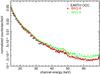 |
Fig. 2 Comparison between the quick (bkgA, red triangles) and the tuned (bkgD, green crosses) backgrounds with the Earth occultation spectra (black squares). The BkgD spectrum is above both the bkgA and the Earth data. The tuned background clearly overpredicts the real NXB, in particular above 35 keV. |
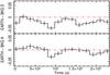 |
Fig. 3 Comparison between light-curves extracted in the 15−50 keV energy range. The Earth light-curves are corrected for the dead time. In the upper panel we show the difference between the Earth and the tuned background (bkgD) light-curves, while in the lower panel we show the difference between the Earth and the quick background (bkgA) light-curves. |
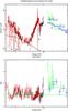 |
Fig. 4 Suzaku XIS-FI (black data points in the electronic version), XIS-BI (red in the electronic version), HXD-PIN (green in the electronic version) and SWIFT-BAT (blue in the electronic version) data of IRAS 04507+0358. Upper panel: unfolded Compton-thin model. The model consists of two thermal emission components (a) and b) components), a scattered component c), a Fe emission line at ~ 6.4 keV d), and an absorbed power-law with a NH fixed to 4 × 1023 cm-2 e). Lower panel: ratio between data and the Compton-thin best-fit model. |
2.4. Broad band X-ray spectral fitting
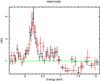 |
Fig. 5 Residuals, with respect to a single power-law, of the XIS data/model (XIS-FI – black data points in the electronic version and XIS-BI-red points in the electronic version) of IRAS 04507+0358 at energies close to the Fe band (observed frame). No iron line is included in the model. |
The XIS, the HXD-PIN, and BAT spectra were fitted simultaneously covering a wide energy range (0.4 − 100 keV) using Xspec version 12.5.0. We tied together XIS, HXD, and BAT parameters. We left the BAT/XIS cross-normalization free to vary, while for the HXD/XIS instruments we assumed a cross-calibration of 1.18 (Manabu et al. 2007; Maeda et al. 20083). In all models described here we used the abundance of Wilms et al. (2000) and the Galactic hydrogen column density along the line of sight (from Dickey & Lockman 1990), NH(Galactic) = 6.7 × 1020 cm-2.
Because the aim of this work is to explore the physical properties of the nuclear regions
of IRAS 04507+0358 (e.g. the NH of the obscuring matter and
the de-absorbed X-ray luminosity of the AGN), a detailed analysis of the spectrum
below 2 keV will not be discussed here. Starting from the results obtained with
XMM-Newton data, we fitted this part with two thermal components. We
left the temperatures free to vary and found that the two temperatures agree well with
those found with XMM-Newton data:
kT and
kT
and
kT .
.
As for the XMM-Newton spectra, to fit the data above 2 keV we used a simple basic model for obscured AGN, i.e. two power-laws with the same slope. One of the two power-laws is absorbed only by Galactic column density and represents the scattered component; the second power-law represents the primary X-ray emission seen through the cold absorber (the putative torus). To reproduce this absorbed power-law, we used the model by Yaqoob 1997 (plcabs in Xspec), which partially takes into account the Compton down-scattering. The Fe emission line was modelled with a Gaussian profile.
Best-fit values of the mildly and heavily Compton-thick AGN models.
Compton-thin hypothesis: as a first step, we tested the
Compton-thin hypothesis by fixing the slope of the power-laws to Γ = 1.9 and the column
density to NH = 4 × 1023 cm-2,
i.e. the values found with the XMM-Newton data (see Fig. 4, χ2/d.o.f. = 527.5/194).
This model provides an overall good representation of the XIS data, but it under-predicts
the HXD-PIN and the BAT data. We left the photon index and the column density free to vary
and found Γ = 1.8 and NH =
5.5
and NH =
5.5 × 1023 cm-2
(χ2/d.o.f. = 334.95/193); but even with these values the
model does not provide a good representation of the emission above 10 keV. Our first
conclusion is that the Compton-thin hypothesis is clearly ruled out by the HXD-PIN and
BAT data.
× 1023 cm-2
(χ2/d.o.f. = 334.95/193); but even with these values the
model does not provide a good representation of the emission above 10 keV. Our first
conclusion is that the Compton-thin hypothesis is clearly ruled out by the HXD-PIN and
BAT data.
Mildly Compton-thick hypothesis: to account for the
prominent Fe emission line in the spectrum and for the excess detected above 10 keV, we
added to the model a component, which represents the emission reflected from neutral
material into our line of sight. In particular, we added the pexrav
model, leaving open the possibility that the reflected emission could be
partially obscured by the torus itself. We fixed the inclination angle to its default
value (i = 60°) and the normalization equal to that of the intrinsic
powerlaw. With the addition of this new component, which we found to be absorbed
(NH = (3.3 ± 0.2) × 1023 cm-2),
the model provides a relatively good fit to the 0.4 − 100 keV spectrum
(χ2/d.o.f. = 265.5/190). We found a BAT/XIS
cross-normalization of 1.1 . The primary X-ray continuum has an
intrinsic slope of Γ = 2.4 ± 0.5 and is absorbed by an NH =
(1.45 ± 0.10) × 1024 cm-2. We found that the scattering fraction
is less than 1%, and the reflection fraction is R =
0.7
. The primary X-ray continuum has an
intrinsic slope of Γ = 2.4 ± 0.5 and is absorbed by an NH =
(1.45 ± 0.10) × 1024 cm-2. We found that the scattering fraction
is less than 1%, and the reflection fraction is R =
0.7 . The slightly steep photon index, which is
also not well constrained (ranging from 1.9 to 2.9), is not so striking if we take the
complexity of the model into account.
. The slightly steep photon index, which is
also not well constrained (ranging from 1.9 to 2.9), is not so striking if we take the
complexity of the model into account.
The Suzaku data confirm the presence of a Fe Kα line at 6.37 ±
0.01 keV (σ < 50 eV), but with a lower equivalent width
(EW = 450 eV) with respect to the value measured
with the XMM-Newton data, although consistent considering the errors.
In order to investigate the presence of other possible features, we inspected the
residuals around 6.4 keV with respect to a single power-law model (see Fig. 5); there are clear residuals, both red- and blue-wards
of the Kα line. Some excesses in the data/model ratio are present around
5.8 keV (observer’s frame) and between 6.5 and 7 keV, while at
E > 7 keV there is a clear drop. While the first excess is most
probably caused by a bad subtraction of the emission lines present in the calibration
source (i.e. Mn Kα1 at 5.899 keV and Mn Kα2 at
5.888 keV), the drop at energies higher than 7 keV is most likely owing to a high level of
the XIS background. Finally, the excess between 6.5 and 7 keV could suggest a second He-
or H-like Fe emission line. In particular, we found that a second narrow
(σ < 50 eV) line centred at ~6.92 keV rest-frame
(EW ~ 100 eV) could be actually present (see Fig. 6) even if it is not statistically required
(χ2/d.o.f. = 255.9/188). This second line could be
associated both to the Fe XXVI Lyα emission line (rest-frame energy
E = 6.96 keV) or to the Fe Kβ emission line
(rest-frame energy E = 7.058 keV) or to a combination of these two lines.
However, we estimated the flux of the 6.92 keV line and found that it is about 15% of the
flux of the Kα line, as is expected for the
Fe Kβ emission line (see e.g. Leahy & Creighton 1993).
eV) with respect to the value measured
with the XMM-Newton data, although consistent considering the errors.
In order to investigate the presence of other possible features, we inspected the
residuals around 6.4 keV with respect to a single power-law model (see Fig. 5); there are clear residuals, both red- and blue-wards
of the Kα line. Some excesses in the data/model ratio are present around
5.8 keV (observer’s frame) and between 6.5 and 7 keV, while at
E > 7 keV there is a clear drop. While the first excess is most
probably caused by a bad subtraction of the emission lines present in the calibration
source (i.e. Mn Kα1 at 5.899 keV and Mn Kα2 at
5.888 keV), the drop at energies higher than 7 keV is most likely owing to a high level of
the XIS background. Finally, the excess between 6.5 and 7 keV could suggest a second He-
or H-like Fe emission line. In particular, we found that a second narrow
(σ < 50 eV) line centred at ~6.92 keV rest-frame
(EW ~ 100 eV) could be actually present (see Fig. 6) even if it is not statistically required
(χ2/d.o.f. = 255.9/188). This second line could be
associated both to the Fe XXVI Lyα emission line (rest-frame energy
E = 6.96 keV) or to the Fe Kβ emission line
(rest-frame energy E = 7.058 keV) or to a combination of these two lines.
However, we estimated the flux of the 6.92 keV line and found that it is about 15% of the
flux of the Kα line, as is expected for the
Fe Kβ emission line (see e.g. Leahy & Creighton 1993).
As reported in Table 1, the best-fit values obtained with both models (one and two emission lines) are consistent within the errors. We refer to these models as mildly Compton-thick AGN models. In Table 1, the lines at ~6.4 and ~6.9 keV are marked as E1 and E2 respectively. The 2−10 keV flux, corrected for the Galactic absorption along the line of sight, is F(2−10 keV) = 2 × 10-12 erg cm-2 s-1 and, once corrected also for the amount of intrinsic absorption, the deabsorbed 2 − 10 keV luminosity of the AGN is 7 × 1043 erg s-1.
To further test the above models, we modelled the two components associated with cold
reflection (the 6.4 keV Gaussian emission and the Compton-scattered continuum from neutral
material) using a single and self-consistent model: reflionx (Ross &
Fabian 2005). In this model, an optically thick
disc is illuminated by a power-law, producing florescence lines and continuum emission.
The parameters include the Fe abundance, ionization parameter ξ (defined
as ξ =
4πFtot/nH,
where Ftot is the total illuminating flux
and nH is the density of the reflector), and the incident
power-law photon index Γ. Because the observed Fe iron Kα emission line
is unresolved in the Suzaku spectrum, no additional velocity broadening was applied to the
reflected spectrum. We found that the data are well reproduced by this model
(χ2/d.o.f. = 226.3/190), confirming the physical consistence
between the measured reflected continuum and the line intensity. In this case the
reflected component is absorbed by NH = (2.7 ± 0.8) ×
1023 cm-2, while the transmitted component is absorbed by a higher
column density NH = (1.3 ± 0.3) ×
1024 cm-2. We found a value for the photon index that is
consistent with the previous ones (Γ = 2.5 ± 0.5) and an ionization parameter
ξ = 29 erg cm s-1 (the lowest value
allowed by the model is ξ = 10 erg cm s-1), in agreement with
iron atoms typically in a low-ionization state corresponding to Fe I − XVII. Best fit
parameters are reported in Table 1 (mildly
Compton-thick AGN models – reflionx).
erg cm s-1 (the lowest value
allowed by the model is ξ = 10 erg cm s-1), in agreement with
iron atoms typically in a low-ionization state corresponding to Fe I − XVII. Best fit
parameters are reported in Table 1 (mildly
Compton-thick AGN models – reflionx).
Finally, we checked the self-consistence of the mildly Compton-thick hypothesis by using the model recently published by Murphy & Yaqoob (2009). They calculated Green’s functions that may be used to produce spectral-fitting routines to model the putative neutral toroidal X-ray reprocessor in AGNs for an arbitrary input spectrum. In their calculation the reprocessed continuum and fluorescent line emission owing to Fe Kα, Fe Kβ and Ni Kα are treated self-consistently. On the basis of the EW obtained for the Fe Kα emission line (~450 eV) by our analysis and by assuming an inclination angle between the observer’s line of sight and the symmetry axis of the torus larger than 60°, the model predicts an NH ≃ 1.5 − 3 × 1024 cm-2. The mildly Compton-thick hypothesis is thus fully supported also by this recent model proposed in the case of neutral toroidal X-ray reprocessor in AGNs.
Heavily Compton-thick hypothesis: for completeness, we also tested the heavily (NH > 1025 cm-2) Compton-thick AGN hypothesis. In this case, the emission is completely dominated by the scattered component at low energies and only by the reflected component (reflionx or pexrav model) at high-energies. By using disc-reflection models (reflionx or pexrav models), we found that this scenario is statistically acceptable. As an example, we report in Fig. 7 and Table 1 the results found with the reflionx model (χ2/d.o.f. = 218.9/189, heavily Compton-thick AGN models – reflionx in Table 1). However, an intrinsic column density higher than 1025 cm-2 is not supported by the model of Murphy & Yaqoob (2009) for Fe Kα EW of the order of 450 eV. Moreover, on the basis of this model, the observed luminosity should be just less than few percents of the intrinsic one, by implying an intrinsic luminosity of L(2−10 keV) ≥ 1045 erg s-1. This value of X-ray luminosity exceeds the infrared luminosity measured for this source (LIR = 2.7 × 1044 erg s-1), which, under the assumption that most of the optical and ultraviolet radiation is absorbed by a dusty torus surrounding the nuclear source, is a good proxy of the bolometric luminosity. Therefore, on the basis of the Murphy & Yaqoob (2009) model, this scenario is not acceptable from the physical point of view.
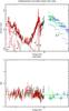 |
Fig. 6 Suzaku XIS-FI (black data points in the electronic version), XIS-BI (red in the electronic version), HXD-PIN (green in the electronic version) and SWIFT-BAT (blue in the electronic version) data of IRAS 04507+0358. Upper panel: unfolded mildly Compton-thick model. The spectral components are a) and b) two thermal emission components; c) scattered AGN component; d) narrow Gaussian line at 6.37 keV; e) absorbed power-law AGN component; f) pure reflection AGN component; g) narrow Gaussian line at ~ 6.9 keV. Lower panel: ratio between data and the mildly Compton-thick best-fit model. |
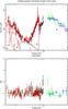 |
Fig. 7 Suzaku XIS-FI (black data points in the electronic version), XIS-BI (red in the electronic version), HXD-PIN (green in the electronic version) and SWIFT-BAT (blue in the electronic version) data of IRAS 04507+0358. Upper panel: the unfolded heavily Compton-thick model (reflionx, see Table 1) is overplotted on the data. The spectral components are a) and b) two thermal emission components; c) scattered AGN component; d) narrow Gaussian line at ~6.9 keV; e) pure reflection AGN component (reflionx). Lower panel: ratio between data and the heavily Compton-thick best-fit model. |
3. Discussion and conclusion
IRAS 04507+0358 was proposed as a new Compton-thick AGN candidate through the diagnostic diagram described in Severgnini et al. (2010). Here, by studying its broad band X-ray spectral properties (0.4 − 100 keV), we confirm the Compton-thick nature of this AGN.
We showed in this paper that with the XMM-Newton and XIS data below 10 keV alone, we could not distinguish between Compton-thin or Compton-thick scenarios. However, the Compton-thin model clearly under-predicts higher energy data. In particular, we found that the favourite scenario is that of a mildly Compton-thick AGN with NH = 1.3−1.5 × 1024 cm-2 and L(2−10 keV) = 5−7 × 1043 erg s-1. This luminosity fully agrees with the observed infrared luminosity and with that predicted for the torus by Fraquelli et al. (2003). These authors, after estimating the rate of the ionizing photons emitted by the AGN and assuming an opening angle of 30° for the ionization cones, predicted an infrared luminosity for the torus of LIR = 5.3 × 1043 erg s-1. This value is about 20% of the infrared luminosity (LIR ≃ 2.7 × 1044 erg s-1, see also Sect. 2). The remaining fraction of the infrared luminosity (2.2 × 1044 erg s-1) is most probably due to star-formation activity and approximately agrees with the soft X-ray luminosity of the thermal components of our source (L(0.5−2 keV) = 2.5 × 1041 erg s-1) considering the L(soft-X) − L(FIR) relation presented in Persic et al. (2004). To estimate the relevant SFR of our source, we adopted the following Kennicutt et al. (1998) relation: SFR = (LFIR/5.8 × 109 L⊙) M⊙ yr-1 and we considered only the infrared luminosity produced by star-formation activity (~2.2 × 1044 erg s-1). We found a SFR of about 10 M⊙ yr-1.
As for the heavily Compton-thick hypothesis, by using disc-reflection models it is possible to well reproduce the broad-band spectrum of IRAS 04507+0358 and to obtain a statistically acceptable fit of the data. In this case, in order not to exceed the bolometric luminosity of the source, the reflection component should be more than 10% of the intrinsic one, which is not supported by the Murphy & Yaqoob (2009) model.
We note that this source could not be found as a possible Compton-thick AGN by using only the data below 10 keV, nor by using the two-dimensional diagnostic tool for reflection-dominated Compton-thick object proposed by Bassani et al. (1999). This latter diagram shows that Compton-thick AGN should be characterized by a high Kα iron line equivalent width (EW > 300 eV) and by a 2 − 10 keV flux normalized to the [OIII] optical-line flux (T parameter) typically lower than 0.5. In this estimate, the [OIII] optical-line flux should be corrected for Galactic and intrinsic extinction. From the X-ray analysis performed on IRAS 04507+0358, we derived for the Fe Kα line an EW of ~450 eV. In order to estimate the T parameter, we considered the [OIII] line flux (already corrected for the Galactic extinction) reported by Cid Fernandes et al. (2001). After the correction for the intrinsic extinction4, we found T = 2, higher than the typical value adopted to select Compton-thick candidates (≪1). This implies that by using 2 − 10 keV data alone and/or diagnostic diagrams based on the Fe Kα line EW vs. 2 − 10 keV to [OIII] flux ratio, a significant fraction of mildly or heavily Compton-thick AGN could be missed. Whereas some examples of Compton-thick AGN with low value of Fe Kα line equivalent width are indeed already present in the literature (e.g. Awaki et al. 2000; Ueda et al. 2007; Braito et al. 2009), IRAS 04507+0358 escapes the diagnostic diagram because of its high value of T. For mildly Compton-thick AGN, this is most probably owing to the large amount of light reflected from the torus (i.e. about 35% of the light emitted by the central source) that increases the continuum in the 2 − 10 keV range. The Compton-thick AGN missed using the Bassani et al. (1999) criteria could be selected by combining infrared information with 2 − 10 keV data and with very hard X-ray follow-ups, as shown by the study presented here. Moreover, our analysis, besides providing a further evidence of the potentiality of the F(2 − 10 keV)/F24 μm vs. HR diagnostic diagram, also shows the importance of using a wide X-ray spectral coverage in order to constrain the intrinsic column density in this type of sources even for mildly Compton-thick AGN.
With the aim of establishing the nature of other Compton-tick AGN candidates found through our diagram, we recently obtained in the Suzaku AO5 call 100 ks of observation for MCG-03-58-007, while the broad-band X-ray analysis for other twelve sources with a SWIFT-BAT counterpart is already ongoing and will be the subject of a forthcoming paper. The final aim is to better constrain and define the Compton-thick AGN population and hence to better estimate their space density.
HR4 is defined using the two following bands: 2−4.5 keV and 4.5−12 keV: HR4 =
 , where CTS are the vignetting corrected
count rates in the energy ranges reported in bracket. See Watson et al. (2009) for details.
, where CTS are the vignetting corrected
count rates in the energy ranges reported in bracket. See Watson et al. (2009) for details.
The screening procedure filter all events within the South Atlantic Anomaly (SAA) as well as with an Earth elevation angle (ELV) < 5° and Earth day-time elevation angles (DYE_ELV) less than 20°. Furthermore also data within 256s of the SAA were excluded from the XIS and within 500s of the SAA for the HXD. Cut-off rigidity (COR) criteria of >8 GV for the HXD data and >6 GV for the XIS were used.
For the intrinsic extinction, we applied the following formula: Fcor[OIII] = Fobs[OIII][(Hα/Hβ)obs/(Hα/Hβ)0]2.94 (Bassani et al. 1999), where Fcor[OIII] is the extinction-corrected flux of [OIII]5007, and Fobs[OIII] the observed flux of [OIII]5007. We used and observed a line ratio of Hα/Hβ = 5.5 (Cid Fernandes et al. 2001) and an intrinsic Balmer decrement of (Hα/Hβ)0 = 3.0.
Acknowledgments
This research has made use of data obtained from the Suzaku satellite, a collaborative mission between the space agencies of Japan (JAXA) and the USA (NASA). Data obtained with XMM-Newton has also been used within this paper, an ESA science mission with instruments and contributions directly funded by ESA Member States and NASA. The authors acknowledge financial support from ASI (grant No. I/088/06/0, COFIS contract and grant No. I/009/10/0). V.B. acknowledge support from the UK STFC research council. We thank Giancarlo Cusumano and Kenji Hamaguchi for their useful
support with the SWIFT-BAT and Suzaku data, respectively. We also thank the anonymous referee for her/his useful comments.
References
- Awaki, H., Ueno, S., & Taniguchi, Y. 2000, AdSpR, 25, 797 [NASA ADS] [Google Scholar]
- Awaki, H., Terashima, Y., Higaki, Y., & Fukazawa, Y. 2009, PASJ, 61, 317 [Google Scholar]
- Ballantyne, D. R., Everett, J. E., & Murray, N. 2006, ApJ, 639, 740 [NASA ADS] [CrossRef] [Google Scholar]
- Bassani, L., Dadina, M., Maiolino, R., et al. 1999, ApJS, 121, 473 [NASA ADS] [CrossRef] [Google Scholar]
- Boldt, E. 1987, Phys. Rep., 146, 215 [NASA ADS] [CrossRef] [Google Scholar]
- Braito, V., Della Ceca, R., Piconcelli, E., et al. 2004, A&A, 420, 79 [NASA ADS] [CrossRef] [EDP Sciences] [Google Scholar]
- Braito, V., Reeves, J. N., Della Ceca, R., et al. 2009, A&A, 504, 53 [NASA ADS] [CrossRef] [EDP Sciences] [Google Scholar]
- Caccianiga, A., Severgnini, P., Braito, V., et al. 2004, A&A, 416, 901 [NASA ADS] [CrossRef] [EDP Sciences] [Google Scholar]
- Cid Fernandes, R., Heckman, T., Schmitt, H., González Delgado, R. M., & Storchi-Bergmann, T. 2001, ApJ, 558, 81 [NASA ADS] [CrossRef] [Google Scholar]
- Comastri, A. 2004, in Supermassive Black Holes in the Distant Universe, ed. A. J. Barger, Astrophys. Space Sci. Libr., 308, 245 [NASA ADS] [CrossRef] [Google Scholar]
- Comastri, A., Iwasawa, K., Gilli, R., et al. 2010, ApJ, 717, 787 [NASA ADS] [CrossRef] [Google Scholar]
- Cusumano, G., La Parola, V., Segreto, A., et al. 2009, AIPC, 1126, 104 [NASA ADS] [CrossRef] [Google Scholar]
- Cusumano, G., La Parola, V., Segreto, A., et al. 2010, A&A, 524, A64 [NASA ADS] [CrossRef] [EDP Sciences] [Google Scholar]
- Della Ceca, R., Ballo, L., Tavecchio, F., et al. 2002, ApJ, 581, 9 [Google Scholar]
- Della Ceca, R., Caccianiga, A., Severgnini, P., et al. 2008a, A&A, 487, 119 [NASA ADS] [CrossRef] [EDP Sciences] [Google Scholar]
- Della Ceca, R., Severgnini, P., Caccianiga, A., et al. 2008b, MmSAI, 79, 65 [Google Scholar]
- Dickey, J. M., & Lockman, F. J. 1990, ARA&A, 28, 215 [NASA ADS] [CrossRef] [MathSciNet] [Google Scholar]
- Fraquelli, H. A., Storchi-Bergmann, T., & Levenson, N. A. 2003, MNRAS, 341, 449 [NASA ADS] [CrossRef] [Google Scholar]
- Gilli, R., Comastri, A., & Hasinger, G. 2007, A&A, 463, 79 [NASA ADS] [CrossRef] [EDP Sciences] [Google Scholar]
- Gruber, D. E., Matteson, J. L., Peterson, L. E., & Jung, G. V. 1999, ApJ, 520, 124 [NASA ADS] [CrossRef] [Google Scholar]
- Kennicutt, R. C. Jr. 1998, ApJ, 498, 541 [NASA ADS] [CrossRef] [Google Scholar]
- Koyama, K., Tsunemi, H., Dotani, T., et al. 2007, PASJ, 59, 23 [Google Scholar]
- Leahy, D. A., & Creighton, J. 1993, MNRAS, 263, 314 [NASA ADS] [CrossRef] [Google Scholar]
- Liedahl, D. A., Osterheld, A. L., & Goldstein, W. H. 1995, ApJ, 438, L115 [NASA ADS] [CrossRef] [Google Scholar]
- Magdziarz, P., & Zdziarski, A. A. 1995, MNRAS, 273, 837 [NASA ADS] [CrossRef] [Google Scholar]
- Mateos, S., Carrera, F. J., Page, M. J., et al. 2010, A&A, 510, A35 [NASA ADS] [CrossRef] [EDP Sciences] [Google Scholar]
- Matt, G. 1996, Proc. Conference Roentgenstrahlung from the Universe, MPE Rep., 263, 479 [Google Scholar]
- Mewe, R., Gronenschild, E. H. B. M., & van den Oord, G. H. J. 1985, A&AS, 62, 197 [Google Scholar]
- Mewe, R., Lemen, J. R., & van den Oord, G. H. J. 1986, A&AS, 65, 511 [NASA ADS] [Google Scholar]
- Mitsuda, K., Bautz, M., Inoue, H., et al. 2007, PASJ, 59, 1 [Google Scholar]
- Murphy, K. D., & Yaqoob, T. 2009, MNRAS, 397, 1549 [NASA ADS] [CrossRef] [Google Scholar]
- Page, K. L., Reeves, J. N., O’Brien, P. T., Turner, M. J. L., & Worrall, D. M. 2004, MNRAS, 353, 133 [NASA ADS] [CrossRef] [Google Scholar]
- Persic, M., Rephaeli, Y., Braito, V., et al. 2004, A&A, 419, 849 [NASA ADS] [CrossRef] [EDP Sciences] [Google Scholar]
- Reeves, J. N., & Turner, M. J. L. 2000, MNRAS, 316, 234 [NASA ADS] [CrossRef] [Google Scholar]
- Risaliti, G., Gilli, R., Maiolino, R., & Salvati, M. 2000, A&A, 357, 13 [NASA ADS] [Google Scholar]
- Ross, R. R., & Fabian, A. C. 2005, MNRAS, 358, 211 [Google Scholar]
- Sanders, D. B., & Mirabel, I. F. 1996, ARA&A, 34, 749 [NASA ADS] [CrossRef] [Google Scholar]
- Segreto, A., Cusumano, G., Ferrigno, C., et al. 2010, A&A, 510, A47 [NASA ADS] [CrossRef] [EDP Sciences] [Google Scholar]
- Severgnini, P., Caccianiga, A., Della Ceca, R., et al. 2010, AIPC, 1248, 511 [NASA ADS] [Google Scholar]
- Strauss, M. A., Huchra, J. P., Davis, M., et al. 1992, ApJS, 83, 29 [NASA ADS] [CrossRef] [EDP Sciences] [Google Scholar]
- Teng, S. H., Veilleux, S., Anabuki, N., et al. 2009, ApJ, 691, 261 [NASA ADS] [CrossRef] [Google Scholar]
- Takahashi, T., Abe, K., Endo, M., et al. 2007, PASJ, 59, 35 [NASA ADS] [CrossRef] [EDP Sciences] [Google Scholar]
- Treister, E., Urry, C. M., & Virani, S. 2009, ApJ, 696, 110 [NASA ADS] [CrossRef] [Google Scholar]
- Tueller, J., Baumgartner, W. H., Markwardt, C. B., et al. 2010, ApJS, 186, 378 [NASA ADS] [CrossRef] [Google Scholar]
- Ueda, Y., Eguchi, S., Terashima, Y., et al. 2007, ApJ, 664, L79 [NASA ADS] [CrossRef] [Google Scholar]
- Vignati, C., Molendi, S., Matt, G., et al. 1999, A&A, 349, L57 [NASA ADS] [Google Scholar]
- Watson, M. G., Schrder, A. C.,Fyfe, D., et al. 2009, A&A, 493, 339 [NASA ADS] [CrossRef] [EDP Sciences] [Google Scholar]
- Wilms, J., Allen, A., & McCray, R. 2000, ApJ, 542, 914 [NASA ADS] [CrossRef] [Google Scholar]
- Yaqoob, T. 1997, ApJ, 479, 184 [NASA ADS] [CrossRef] [Google Scholar]
All Tables
All Figures
|
Fig. 1 XMM-Newton (MOS1 – black data points in the electronic version and MOS2 – red data points in the electronic version) unfolded spectrum of IRAS 04507+0358 fitted with a Compton-thin (left panel) and a Compton-thick model (right panel). In the lower panels the ratio between data and best-fit models are shown. In the Compton-thin hypothesis, the data are best reproduced by two thermal emission components (a), b)) plus a power-law absorbed only by the Galactic column density (scattering component, c)) and a power-law absorbed by a high column density (NH = (4 ± 2) × 1023 cm-2) absorber e). The two power-laws have the same Γ fixed to 1.9. A prominent iron line is also present d). A similarly good fit could be obtained by using a cold reflection component instead of the absorbed power-law (component e) in the right panel). |
| In the text | |
|
Fig. 2 Comparison between the quick (bkgA, red triangles) and the tuned (bkgD, green crosses) backgrounds with the Earth occultation spectra (black squares). The BkgD spectrum is above both the bkgA and the Earth data. The tuned background clearly overpredicts the real NXB, in particular above 35 keV. |
| In the text | |
|
Fig. 3 Comparison between light-curves extracted in the 15−50 keV energy range. The Earth light-curves are corrected for the dead time. In the upper panel we show the difference between the Earth and the tuned background (bkgD) light-curves, while in the lower panel we show the difference between the Earth and the quick background (bkgA) light-curves. |
| In the text | |
|
Fig. 4 Suzaku XIS-FI (black data points in the electronic version), XIS-BI (red in the electronic version), HXD-PIN (green in the electronic version) and SWIFT-BAT (blue in the electronic version) data of IRAS 04507+0358. Upper panel: unfolded Compton-thin model. The model consists of two thermal emission components (a) and b) components), a scattered component c), a Fe emission line at ~ 6.4 keV d), and an absorbed power-law with a NH fixed to 4 × 1023 cm-2 e). Lower panel: ratio between data and the Compton-thin best-fit model. |
| In the text | |
|
Fig. 5 Residuals, with respect to a single power-law, of the XIS data/model (XIS-FI – black data points in the electronic version and XIS-BI-red points in the electronic version) of IRAS 04507+0358 at energies close to the Fe band (observed frame). No iron line is included in the model. |
| In the text | |
|
Fig. 6 Suzaku XIS-FI (black data points in the electronic version), XIS-BI (red in the electronic version), HXD-PIN (green in the electronic version) and SWIFT-BAT (blue in the electronic version) data of IRAS 04507+0358. Upper panel: unfolded mildly Compton-thick model. The spectral components are a) and b) two thermal emission components; c) scattered AGN component; d) narrow Gaussian line at 6.37 keV; e) absorbed power-law AGN component; f) pure reflection AGN component; g) narrow Gaussian line at ~ 6.9 keV. Lower panel: ratio between data and the mildly Compton-thick best-fit model. |
| In the text | |
|
Fig. 7 Suzaku XIS-FI (black data points in the electronic version), XIS-BI (red in the electronic version), HXD-PIN (green in the electronic version) and SWIFT-BAT (blue in the electronic version) data of IRAS 04507+0358. Upper panel: the unfolded heavily Compton-thick model (reflionx, see Table 1) is overplotted on the data. The spectral components are a) and b) two thermal emission components; c) scattered AGN component; d) narrow Gaussian line at ~6.9 keV; e) pure reflection AGN component (reflionx). Lower panel: ratio between data and the heavily Compton-thick best-fit model. |
| In the text | |
Current usage metrics show cumulative count of Article Views (full-text article views including HTML views, PDF and ePub downloads, according to the available data) and Abstracts Views on Vision4Press platform.
Data correspond to usage on the plateform after 2015. The current usage metrics is available 48-96 hours after online publication and is updated daily on week days.
Initial download of the metrics may take a while.