| Issue |
A&A
Volume 528, April 2011
|
|
|---|---|---|
| Article Number | A27 | |
| Number of page(s) | 16 | |
| Section | Planets and planetary systems | |
| DOI | https://doi.org/10.1051/0004-6361/201015809 | |
| Published online | 22 February 2011 | |
Tidal obliquity evolution of potentially habitable planets
1
Astrophysikalisches Institut Potsdam (AIP),
An der Sternwarte 16,
14482
Potsdam,
Germany
e-mail: rheller@aip.de
2
Hamburger Sternwarte, Graduiertenkolleg 1351 “Extrasolar Planets
and their Host Stars” of the Deutsche
Forschungsgesellschaft, Germany
3
École Normale Supérieure de Lyon, CRAL (CNRS), Université Lyon,
46 allée d’Italie,
69364
Lyon Cedex 07,
France
e-mail: jeremy.leconte@ens-lyon.fr
4
University of Washington, Dept. of Astronomy, Seattle, WA
98195,
USA
e-mail: rory@astro.washington.edu
5 Virtual Planetary Laboratory, USA
Received:
23
September
2010
Accepted:
10
January
2011
Context. Stellar insolation has been used as the main constraint on a planet’s potential habitability. However, as more Earth-like planets are discovered around low-mass stars (LMSs), a re-examination of the role of tides on the habitability of exoplanets has begun. Those studies have yet to consider the misalignment between a planet’s rotational axis and the orbital plane normal, i.e. the planetary obliquity.
Aims. This paper considers the constraints on habitability arising from tidal processes due to the planet’s spin orientation and rate. Since tidal processes are far from being understood we seek to understand differences between commonly used tidal models.
Methods. We apply two equilibrium tide theories – a constant-phase-lag model and a constant-time-lag model – to compute the obliquity evolution of terrestrial planets orbiting in the habitable zones around LMSs. The time for the obliquity to decrease from an Earth-like obliquity of 23.5° to 5°, the “tilt erosion time”, is compared to the traditional insolation habitable zone (IHZ) in the parameter space spanned by the semi-major axis a, the eccentricity e, and the stellar mass Ms. We also compute tidal heating and equilibrium rotation caused by obliquity tides as further constraints on habitability. The Super-Earth Gl581 d and the planet candidate Gl581 g are studied as examples for these tidal processes.
Results. Earth-like obliquities of terrestrial planets in the IHZ around stars with masses ≲ 0.25 M⊙ are eroded in less than 0.1 Gyr. Only terrestrial planets orbiting stars with masses ≳ 0.9 M⊙ experience tilt erosion times larger than 1 Gyr throughout the IHZ. Tilt erosion times for terrestrial planets in highly eccentric orbits inside the IHZ of solar-like stars can be ≲ 10 Gyr. Terrestrial planets in the IHZ of stars with masses ≲ 0.25 M⊙ undergo significant tidal heating due to obliquity tides, whereas in the IHZ of stars with masses ≳ 0.5 M⊙ they require additional sources of heat to drive tectonic activity. The predictions of the two tidal models diverge significantly for e ≳ 0.3. In our two-body simulations, Gl581 d’s obliquity is eroded to 0° and its rotation period reached its equilibrium state of half its orbital period in < 0.1 Gyr. Tidal surface heating on the putative Gl581 g is ≲ 150 mW/m2 as long as its eccentricity is smaller than 0.3.
Conclusions. Obliquity tides modify the concept of the habitable zone. Tilt erosion of terrestrial planets orbiting LMSs should be included by atmospheric modelers. Tidal heating needs to be considered by geologists.
Key words: planets and satellites: dynamical evolution and stability / celestial mechanics / planet-star interactions / astrobiology / stars: low-mass / planets and satellites: tectonics
© ESO, 2011
1. Introduction
1.1. The role of obliquity for a planetary atmosphere
The obliquity of a planet, i.e. the angle ψp between its spin axis and the orbital normal, is a crucial parameter for the possible habitability of a planet. On Earth, the orbital angular momentum of the Moon stabilizes ψp at roughly 23.5° against chaotic perturbations from the other solar system planets (Laskar et al. 1993). This steady tilt causes seasons and, together with the rotation period of 1 d, assures a smooth temperature distribution over the whole globe with maximum variations of 150 K. Measurements of oxygen isotope ratios of benthic foraminifera (δ18Ob) in deep-sea sediments suggest that changes in the Earth’s obliquity have caused phases of glaciations on a global scale (Drysdale et al. 2009). In general, the coupled evolution of eccentricity (e) and obliquity has a fundamental impact on the global climate of terrestrial planets (Dressing et al. 2010), with higher obliquities rendering planets habitable at larger semi-major axes. Williams & Kasting (1997) investigated varying obliquities for Earth and concluded that a substantial part of the Earth would not be tolerable for life if its obliquity were as high as 90°. Hunt (1982) studied the impact of zero obliquity on the temperature distribution on Earth’s and finds a global contraction of the inhabitable area on Earth for such a case. Thus, both extremely high and very low obliquities pose a threat for a planet’s habitability. A discussion of the prospects of eukaryotic life to survive a snowball Earth is given by Hoffmann & Schrag (2002).
For ψp ≲ 5° the habitability of a terrestrial planet might crucially be hindered. Decreasing obliquities induce less seasonal variation of solar insolation between higher and lower latitudes. Thus, winters get milder and summers become cooler. Given that cool summer temperatures turn out to be more important than cold winters for the emergence of continental ice sheets, smaller tilt angles lead to more glaciation. As a consequence, the temperature contrast between polar and equatorial regions gets very strong (Spiegel et al. 2009), possibly leading to a collapse of the potential atmosphere (priv. comm. with Frank Selsis), which freezes out at the poles or evaporates at the equator.
1.2. Variations and lockings of the obliquity
It is generally assumed that planets form in a disk around the host star. It was thought that this disk is coplanar with the equatorial plane of the star and the planet’s spin axis is aligned with the orbital normal. However, observational evidence points towards a more complex formation scenario, where the stellar obliquity, i.e. the misalignment between the stellar rotation axis and the orbital plane normal, depends on stellar and planetary mass (Winn et al. 2010) as well as on the influence of perturbing bodies (Fabrycky & Tremaine 2007). Furthermore, the spin axes of planets can experience significant re-orientations by giant impacts during the planetary formation period. Thus, the spin axes of the planets themselves are not necessarily perpendicular to the orbital plane. The obliquity ψp can have any orientation with values 0 ≤ ψp ≤ 180° (Agnor et al. 1999; Chambers 2001; Kokubo & Ida 2007; Miguel & Brunini 2010), where a rotation prograde with the orbital motion means 0 ≤ ψp ≤ 90° and ψp > 90° defines a retrograde planet rotation.
In the course of the planet’s lifetime, this possible spin-orbit misalignment can be subject to lockings or severe perturbations, e.g. by a third or more bodies inducing chaotic interaction (Laskar & Joutel 1993; Laskar et al. 1993) or Milanković cycles (Milanković 1941; Spiegel et al. 2010); the putative presence of a moon that stabilizes the planet’s obliquity as on Earth (Neron de Surgy & Laskar 1997); a perturber that pumps the planet into Cassini states (Gladman et al. 1996) or drives the Kozai mechanism by leverage effects (Kozai 1962; Fabrycky & Tremaine 2007; Migaszewski & Gozdziewski 2010). In the case of Gl581 d, e.g., orbital oscillations due to gravitational interactions occur with timescales of 103 years (Barnes et al. 2008).
Non-spherical, inhomogeneous planets may have their spin state modified by gravitational interactions with other bodies in the planetary system, assuming the system is not coplanar. These mass asymmetries provide a leverage that torques the planet. The amplitudes and frequencies of the variations are complex functions of the orbital evolution of the system as a whole, as the distances between all the planets, and hence the resulting gravitational torques, are constantly changing. In many cases, such as on Mars, the obliquity evolution is chaotic.
Eccentricity oscillations in the Gl581 system occur on 103 yr timescales (Barnes et al. 2008). Thus, bodily obliquities will be significant if tidal processes between the planet and its host star are too weak to align the spin with the orbital plane normal on shorter time scales (Barnes et al. 2010b). So far, the relative inclinations between most of the members of the Gl581 system are unknown, and hence the magnitudes of the torques cannot be estimated at present. Only the mutual inclination of υ And A c and d has just been measured to be nearly 30° (McArthur et al. 2010), suggesting that large variations may be possible among exoplanets. Moreover, the high eccentricity of Gl581 d (Mayor et al. 2009), likely induced by planet-planet scattering (Marzari & Weidenschilling 2002), suggests a significant inclination between the orbits of planet e through f. Therefore, we should expect that the obliquities of the Gl581 planets are more likely to be controlled by interactions among themselves, rather than tidal interactions with the star.
1.3. Tidal effects induced by planetary obliquity
Tidal interaction between a planet and its host star may alter the orbital and structural characteristics of the bodies. The evolution of the planet’s semi-major axis a, eccentricity e, its rotation period Prot, and ψp can put constraints on its habitability. In the long term, as discussed below, tidal effects reduce a planet’s initial obliquity. We call this effect “tilt erosion”. Given all the dependencies of a planet’s climate on the body’s obliquity, as described above, an investigation of tilt erosion is required.
Tidal processes imply exchange of orbital and/or rotational momentum between the bodies. The total angular momentum is conserved but friction in the objects transforms orbital energy into heat, which is released in the two bodies. This effect, called “tidal heating”, can alter the planet’s geology and thus also constrains habitability. On the rocky moon Io e.g., surface heating rates of 2 W/m2 (Spencer et al. 2000), excited by tidal distortions from Jupiter, are related to global volcanism. It is currently not known if a planet’s geophysical activity is controlled by the surface heat flux (Segatz et al. 1988; Spohn 1991; Stamenkovic et al. 2009; Plesa & Breuer 2009) – or vice versa. Instead, tectonic activity on a planet may be determined by the volumetric heating rate or the degree of lithospheric fracturing or as the case may be, but these properties are currently not measurable remotely. While surface tidal heating rates may set an upper limit for a planet’s habitability, they may also provide a lower limit. Here, we think of such planets, where tidal heating is the major source of inner energy that could drive geologic activity. In the solar system we find this constellation for various moons orbiting the giant planets, such as on Io and Europa around Jupiter, Enceladus orbiting Saturn, and Triton escorting Neptune.
The role of plate tectonics for the emergence and survival of life has been discussed, e.g. in Kasting & Catling (2003) and Gaidos et al. (2005). In the terrestrial planets of the solar system, as well as in the Moon, the radiogenic decay of long-lived isotopes 40 K, 232 Th, 235 U, and 238 U provided an energy source that drove or drives structural convection (Spohn 1991; Gaidos et al. 2005). The current mean surface output of radioactive decay on Earth is ≈ 0.04 W/m2 while the global mean heat flow is ≈ 0.086 W/m2 (see Sect. 6 and Fig. 8 in Zahnle et al. 2007). While an Earth-sized object obviously can maintain its radiogenic heat source for several Gyr, the heat flow in a Mars-sized planet decreases much more rapidly. Early Mars tectonically froze when its surface heating rates, driven by radiogenic processes and not by tides, dropped below roughly 0.04 W/m2 (Francis & Wood 1982; Williams et al. 1997). Currently its surface rates due to radiogenic processes are ≈ 0.03 W/m2 (Spohn 1991). Obliquity tides may deliver a source of energy sufficient to drive tectonic mechanisms (Williams et al. 1997) of exoplanets near or in the IHZ of LMSs.
Besides tilt erosion, another threat for a planet’s habitability emerges from “tidal equilibrium rotation”. If zero eccentricity coincides with zero obliquity, the tidal equilibrium rotation period of a planet will equal its orbital period. In the reference system of the synchronously rotating planet, the host star is then static. This configuration could destabilize the planet’s atmosphere, where one side is permanently heated and the other one dark. As we will show, synchronous rotation is only possible if sin(ψp) = 0.
1.4. Obliquities and the insolation habitable zone
Previous studies (Barnes et al. 2008; Jackson et al. 2008; Barnes et al. 2009, 2010a; Henning et al. 2009) investigated the impact of tidal heating and orbital evolution on the habitability of exoplanets but not the effect of tilt erosion. We investigate here the timescales for tilt erosion of terrestrial planets orbiting main-sequence stars with masses as high as 1 M⊙. M dwarf stars are possible hosts for habitable planets (Tarter et al. 2007), they contribute by far the majority of stars in the solar neighborhood, and transit signatures of extrasolar planets can be distinguished most easily in front of small – thus low-mass – stars. We calculate tilt erosion times in the parameter space of e, a, and stellar mass Ms. These regions are then compared with the traditional insolation habitable zone (IHZ). This zone is commonly thought of as the orbital distance between the planet and its host star, where stellar insolation is just adequate to allow the existence of liquid water on the planetary surface. While the first attempts of this concept (Kasting et al. 1993) were primarily based on experience from the solar system, recent approaches include further effects such as orbital eccentricity, tidal evolution, and the atmosphere of the planet (Selsis et al. 2007; Barnes et al. 2008; Spiegel et al. 2009). In addition to the tidal obliquity evolution of potentially habitable planets, we also examine the amount of tidal heating induced by obliquities.
Our models applied below describe the interaction of two bodies: a star and a planet. We neglect relativistic effects and those arising from the presence of more bodies and assume tidal interaction of the planet with its host star as the dominant gravitational process. Our approach does not invoke the geological or rheological response of the body to tidal effects.
This article is structured as follows: after this introduction, we devote Sect. 2 to the two models of equilibrium tide and we motivate our choice of parameter values. In Sect. 3 we describe the constraints that may arise from tidal obliquity processes on the habitability of terrestrial planets, i.e. tilt erosion, tidal heating, and equilibrium rotation. Section 4 is dedicated to the results, in particular to a comparison with the traditional IHZ, while we discuss the results in Sect. 5. In Sect. 6 we conclude.
2. Methods
2.1. Parametrizing tidal dissipation
2.1.1. Equilibrium tide theories
Most current theories for the tidal evolution of celestial bodies are derived from the assumption of equilibrium tides, originally developed by Darwin (1879). This model assumes that the gravitational potential of the tide raiser can be expressed as the sum of Legendre polynomials Pl and it is assumed that the elongated equilibrium shape of the perturbed body is slightly misaligned with respect to the line which connects the two centers of masses. This misalignment is due to dissipative processes within the deformed body and it leads to a secular evolution of the orbital elements of the system. The actual shape of a tidally deformed body is difficult to calculate directly, as it is a function of both the gradient of the gravitational force across the body’s diameter, as well as the body’s internal structure and composition. Initial attempts to model tidal evolution therefore made the assumption that the shape of a body could be well-represented by a superposition of surface waves with different frequencies and amplitudes. This approach does a reasonable job of reproducing the measurable tidal effects on the Earth-Moon and Jupiter-Io systems, but its applicability to large eccentricities ( ≳ 0.3) is dubious (see e.g. Ferraz-Mello et al. 2008; Greenberg 2009). This “lag-and-add” method consists of a Fourier decomposition of the tidal forcing, where small tidal phase lags εl(χl), or geometrical lags δl(χl) = εl(χl)/2 (MacDonald 1964), are added for each frequency χl. The key flaw of this theory emerges from the fact that the “lag-and-add” procedure of polynomials Pl is only reasonable for a tight range of tidal frequencies (Greenberg 2009).
As long as the amplitude of tidal deformation of the body is small, deviations from the
equilibrium shape are assumed to be proportional to the distorting force (Love 1927). By analogy with the driven harmonic
oscillator, the tidal dissipation function Q has been introduced, where
 (1)(Efroimsky & Williams 2009). This parameter is a measure of
the tidal energy dissipated in one cycle (see Appendix of Efroimsky & Williams 2009, for a complete discussion).
(1)(Efroimsky & Williams 2009). This parameter is a measure of
the tidal energy dissipated in one cycle (see Appendix of Efroimsky & Williams 2009, for a complete discussion).
To this point, no assumptions have been made about the frequency dependence of the lag.
It is hard to constrain empirically and depends on the structure and composition of the
deformed body. For the Earth, seismic data argue for
 , with
0.2 ≲ α ≲ 0.4 and
yr-1 ≲ χl ≲ 107 Hz
(Efroimsky & Lainey 2007b,a). For gaseous planets and for stars, numerical
simulations and analytical studies find a complex response spectrum, which is extremely
sensitive to the size and depth of the convective and radiative layers (Ogilvie & Lin 2004; Goodman & Lackner 2009). To derive simple estimates of the
effects of tidal dissipation on the orbital evolution, two main prescriptions for the
lag of the equilibrium have been established over the years.
, with
0.2 ≲ α ≲ 0.4 and
yr-1 ≲ χl ≲ 107 Hz
(Efroimsky & Lainey 2007b,a). For gaseous planets and for stars, numerical
simulations and analytical studies find a complex response spectrum, which is extremely
sensitive to the size and depth of the convective and radiative layers (Ogilvie & Lin 2004; Goodman & Lackner 2009). To derive simple estimates of the
effects of tidal dissipation on the orbital evolution, two main prescriptions for the
lag of the equilibrium have been established over the years.
One of these two approaches is called the “constant phase lag” (CPL) model. Motivated
by the slow variation of the dissipation function for the Earth,
εl can be considered as constant for
each tidal frequency, thus  (Gerstenkorn 1955; Goldreich & Soter 1966; Kaula
1964; Peale 1999; Ferraz-Mello et al. 2008). On the one hand, this procedure seems to
fairly reproduce the rheology of the Earth. On the other hand, it results in
discontinuities when the tidal frequency is close to zero, which is the case for nearly
synchronized exoplanets.
(Gerstenkorn 1955; Goldreich & Soter 1966; Kaula
1964; Peale 1999; Ferraz-Mello et al. 2008). On the one hand, this procedure seems to
fairly reproduce the rheology of the Earth. On the other hand, it results in
discontinuities when the tidal frequency is close to zero, which is the case for nearly
synchronized exoplanets.
The other approach, termed “constant time lag” (CTL) model, introduces the relation
 , which is
equivalent to a fixed time lag τ between the tidal bulge and the line
connecting the centers of the two bodies under consideration (Darwin 1879; Singer 1972;
Mignard 1979, 1980; Hut 1981; Eggleton et al. 1998). This choice coincides with the visco-elastic
limit (Greenberg 2009). It does not produce
discontinuities for vanishing tidal frequencies, as they occur for the CPL model in the
case of synchronous rotation, and it allows for a complete analytical calculation of the
tidal effects without any assumption on the eccentricity (Leconte et al. 2010). This is particularly relevant for the study of
exoplanets in close orbits, which often turn out to be highly eccentric. However, the
key flaw in this case is that coupling between the modes has been ignored.
, which is
equivalent to a fixed time lag τ between the tidal bulge and the line
connecting the centers of the two bodies under consideration (Darwin 1879; Singer 1972;
Mignard 1979, 1980; Hut 1981; Eggleton et al. 1998). This choice coincides with the visco-elastic
limit (Greenberg 2009). It does not produce
discontinuities for vanishing tidal frequencies, as they occur for the CPL model in the
case of synchronous rotation, and it allows for a complete analytical calculation of the
tidal effects without any assumption on the eccentricity (Leconte et al. 2010). This is particularly relevant for the study of
exoplanets in close orbits, which often turn out to be highly eccentric. However, the
key flaw in this case is that coupling between the modes has been ignored.
We use two of the most recent studies on equilibrium tides, one representing the family
of CPL models (Ferraz-Mello et al. 2008, FM08 in
the following) and one representing the family of CTL models (Leconte et al. 2010, Lec10 in the following), to simulate the tidal
evolution of terrestrial planets around LMSs. When comparing the values of the key tidal
parameters in these two theories, i.e. Q for the CPL model and
τ for the CTL model, we recall that both models yield similar results
in the limit of ψp → 0 and
e → 0. For a non-synchronously rotating object, the semi-diurnal
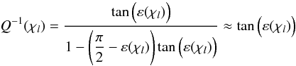
tides dominate and Eq. (1) yields
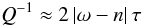 (2)for the leading
frequency
χl = 2 | ω − n | .
In the case of a nearly synchronous planet, annual tides dominate, thus
χl = n and
Q-1 ≈ n τ (see Lec10
for a detailed discussion).
(2)for the leading
frequency
χl = 2 | ω − n | .
In the case of a nearly synchronous planet, annual tides dominate, thus
χl = n and
Q-1 ≈ n τ (see Lec10
for a detailed discussion).
2.1.2. Response in celestial bodies
In this paper, particular attention is drawn to the evolution of the spin-orbit
orientation and the rotation period. As test objects we choose an Earth-mass planet and
a terrestrial Super-Earth with
Mp = 10 MEarth, where
Mp is the mass of the planet and
MEarth is the mass of the Earth. Terrestrial bodies of
such masses may have a variety of compositions (Bond
et al. 2010), thus their response to tidal processes can vary. Against this
background, we choose a value of 0.5 for the radius of gyration
 of the terrestrial planet, where Ip is the moment of inertia
around the rotational axis. The relationship between Mp and
the planetary radius Rp is taken as
Rp = (Mp/MEarth)0.27 × REarth
(Sotin et al. 2007). For both the Earth analog
and the Super-Earth we choose a tidal dissipation value of
Q = 100, owing to the values for Earth given by Ray et al. (2001) and Henning et al. (2009). Measurements of the Martian dissipation function
QMars = 79.91 ± 0.69 (Lainey et al. 2007), as well as estimates for Mercury, where
QMercury < 190, Venus, with
QVenus < 17 (Goldreich & Soter 1966), Io, implying
QIo < 100 (Peale et al. 1979; Peale & Greenberg
1980; Segatz et al. 1988), and the Moon,
with QMoon = 26.5 ± 1 (Dickey et al. 1994), indicate a similar order of magnitude for the tidal
dissipation function of all terrestrial bodies. For Super-Earths at distances
< 1 AU to their host star, the atmospheres are assumed to be no more massive
than 10-1 Mp (Fig. 6 in Rafikov 2006), typically much less massive. Although thermal tides
can have an effect on a planet’s tidal evolution (as shown for Venus by Ingersoll & Dobrovolskis 1978), we neglect
their contribution to the tidal evolution of our test bodies for simplicity. Over the
course of the numerical integrations we use a fixed value for Q. In
real bodies, Q is a function of the bodies′
rigidity μ, viscosity η, and
temperature T (Segatz et al.
1988; Fischer & Spohn 1990). A
comprehensive tidal model would couple the orbital and structural evolution of the
bodies since small perturbations in T can result in large variations in
Q (Segatz et al. 1988; Mardling & Lin 2002; Efroimsky & Lainey 2007b). To estimate the impact on our
results arising from uncertainties in Q, we will show an example where
the tidal dissipation function for an Earth-mass planet is varied by a factor of two, to
values of 50 and 200, and the dissipation value for the Super-Earth is varied by factor
of 5, to values of 20 and 500. Henning et al.
(2009) sum up estimates for Q and the Love number of degree 2,
k2, for planets in the solar system. They find
k2 = 0.3 and Q = 50 the most
reasonable choice for an Earth-like planet (for the relationship between
Q and k2 see Henning et al. 2009). We take
Qp = 100 and
k2 = 0.3 (Yoder
1995) for the terrestrial planets, consistent with our previous studies. With
Q′ = 3/2 × Q/k2
we thus have
of the terrestrial planet, where Ip is the moment of inertia
around the rotational axis. The relationship between Mp and
the planetary radius Rp is taken as
Rp = (Mp/MEarth)0.27 × REarth
(Sotin et al. 2007). For both the Earth analog
and the Super-Earth we choose a tidal dissipation value of
Q = 100, owing to the values for Earth given by Ray et al. (2001) and Henning et al. (2009). Measurements of the Martian dissipation function
QMars = 79.91 ± 0.69 (Lainey et al. 2007), as well as estimates for Mercury, where
QMercury < 190, Venus, with
QVenus < 17 (Goldreich & Soter 1966), Io, implying
QIo < 100 (Peale et al. 1979; Peale & Greenberg
1980; Segatz et al. 1988), and the Moon,
with QMoon = 26.5 ± 1 (Dickey et al. 1994), indicate a similar order of magnitude for the tidal
dissipation function of all terrestrial bodies. For Super-Earths at distances
< 1 AU to their host star, the atmospheres are assumed to be no more massive
than 10-1 Mp (Fig. 6 in Rafikov 2006), typically much less massive. Although thermal tides
can have an effect on a planet’s tidal evolution (as shown for Venus by Ingersoll & Dobrovolskis 1978), we neglect
their contribution to the tidal evolution of our test bodies for simplicity. Over the
course of the numerical integrations we use a fixed value for Q. In
real bodies, Q is a function of the bodies′
rigidity μ, viscosity η, and
temperature T (Segatz et al.
1988; Fischer & Spohn 1990). A
comprehensive tidal model would couple the orbital and structural evolution of the
bodies since small perturbations in T can result in large variations in
Q (Segatz et al. 1988; Mardling & Lin 2002; Efroimsky & Lainey 2007b). To estimate the impact on our
results arising from uncertainties in Q, we will show an example where
the tidal dissipation function for an Earth-mass planet is varied by a factor of two, to
values of 50 and 200, and the dissipation value for the Super-Earth is varied by factor
of 5, to values of 20 and 500. Henning et al.
(2009) sum up estimates for Q and the Love number of degree 2,
k2, for planets in the solar system. They find
k2 = 0.3 and Q = 50 the most
reasonable choice for an Earth-like planet (for the relationship between
Q and k2 see Henning et al. 2009). We take
Qp = 100 and
k2 = 0.3 (Yoder
1995) for the terrestrial planets, consistent with our previous studies. With
Q′ = 3/2 × Q/k2
we thus have  . For the CPL model of
FM08 we assume the dynamical Love number of the ith body,
kd,i, to be equal to
k2,i. For the star we take
Qs = 105 (Heller et al. 2010).
. For the CPL model of
FM08 we assume the dynamical Love number of the ith body,
kd,i, to be equal to
k2,i. For the star we take
Qs = 105 (Heller et al. 2010).
The tidal time lag τ of the Earth with respect to the Moon as a tide raiser has been estimated to 638 s (Neron de Surgy & Laskar 1997) and ≈ 600 s (Lambeck 1977, p. 562 therein). We apply the more recent value of 638 s to model the tidal evolution of the terrestrial planets with the CTL model and apply a fixed τs = 1/(Qsnini), where nini is the orbital mean motion at the beginning of the integration. Over the course of the integration, τp and τs are fixed. For those examples, where we vary Qp in the CPL model, the tidal time lag will be adapted to τp = 638 s × 100/Qp since roughly τp ∝ 1/Qp.
Empirical values for Qp and τp are mostly found by backwards integrations of the secular motions of the respective bodies, where initial conditions need to be assumed (examples for the derivation of Q values in the Solar System are given by Goldreich & Soter 1966), or by precise measurements of the evolution of the orbital elements. There is no general conversion between Qp and τp. Only if e = 0 and ψp = 0, when merely a single tidal lag angle εp exists, then the approximation Qp ≈ 1/εp ≈ 1/(2 |n − ωp| τp) applies – as long as n − ωp remains unchanged. Hence, a dissipation value for an Earth-like planet of Qp = 100 is not equivalent to a tidal time lag of 638 s, so the results for the tidal evolution will intrinsically differ among the CPL and the CTL model. However, both choices are common for the respective model.
2.2. Equilibrium tide with constant phase lag (CPL)
The reconsideration of Darwin’s theory (Darwin
1879, 1880) by FM08 is restricted to low
eccentricities and obliquities. To compute the orbital evolution of the star-planet system
self-consistently, we numerically integrate a set of six coupled differential equations
for the eccentricity e, the semi-major axis a, the two
rotational frequencies ωi
(i ∈ { s,p } , where the subscripts “s” and “p” refer to the star and
the planet, respectively), and the two obliquities
ψi given by ![\begin{eqnarray} \label{equ:e_FM} \frac{\mathrm{d}e}{\mathrm{d}t} &=& - \frac{ae}{8 G M_1 M_2} \sum_{i \, \neq \, j}Z'_i \left( 2\varepsilon_{0,i} - \frac{49}{2}\varepsilon_{1,i} + \frac{1}{2}\varepsilon_{2,i} + 3\varepsilon_{5,i} \right) \\ \frac{\mathrm{d}a}{\mathrm{d}t} &=& \frac{a^2}{4 G M_1 M_2} \sum_{i \, \neq \, j} Z'_i {\Bigg (} 4\varepsilon_{0,i} + e^2{\Big [} -20\varepsilon_{0,i} + \frac{147}{2}\varepsilon_{1,i} \nonumber\\ && + \frac{1}{2}\varepsilon_{2,i} - 3\varepsilon_{5,i} {\Big ]} -4\sin^2(\psi_i){\Big [}\varepsilon_{0,i}-\varepsilon_{8,i}{\Big ]}{\Bigg )} \\ \frac{\mathrm{d}\omega_i}{\mathrm{d}t} &=& - \frac{Z'_i}{8 M_i r_{\mathrm{g},i}^2 R_i^2 n} {\Bigg (}4\varepsilon_{0,i} + e^2{\Big [} -20\varepsilon_{0,i} + 49\varepsilon_{1,i} + \varepsilon_{2,i} {\Big ]} \nonumber\\\label{equ:psi_FM} & &+ 2\sin^2(\psi_i) {\Big [} -2\varepsilon_{0,i} + \varepsilon_{8,i} + \varepsilon_{9,i} {\Big ]} {\Bigg )} \\ \frac{\mathrm{d}\psi_i}{\mathrm{d}t} & =& \frac{Z'_i \sin(\psi_i)}{4 M_i r_{\mathrm{g},i}^2 R_i^2 n \omega_i} {\Bigg (} {\Big [} 1-\xi_i {\Big ]}\varepsilon_{0,i} + {\Big [} 1+\xi_i {\Big ]}{\Big \{}\varepsilon_{8,i}-\varepsilon_{9,i}{\Big \}} {\Bigg )} . \end{eqnarray}](/articles/aa/full_html/2011/04/aa15809-10/aa15809-10-eq97.png) In
these equations,
In
these equations,  stands for
 (7)
(7) , G is
Newton’s gravitational constant, n is the orbital mean motion or orbital
frequency, Mi is the mass of the
ith body, and Ri its mean
radius. The algebraic signs of the tidal phase lags are given by
, G is
Newton’s gravitational constant, n is the orbital mean motion or orbital
frequency, Mi is the mass of the
ith body, and Ri its mean
radius. The algebraic signs of the tidal phase lags are given by ![\begin{eqnarray} \label{equ:epsilon} \nonumber \varepsilon_{0,i} & =& \Sigma(2 \omega_i - 2 n)\\ \nonumber \varepsilon_{1,i} & =& \Sigma(2 \omega_i - 3 n)\\ \nonumber \varepsilon_{2,i} & =& \Sigma(2 \omega_i - n)\\ \nonumber \varepsilon_{5,i} & =& \Sigma(n)\\ \nonumber \varepsilon_{8,i} & =& \Sigma(\omega_i - 2 n)\\ \varepsilon_{9,i} & =& \Sigma(\omega_i) ,\\[-2mm] \nonumber \end{eqnarray}](/articles/aa/full_html/2011/04/aa15809-10/aa15809-10-eq105.png) (8)with
Σ(x) the sign of any physical quantity x, thus
Σ(x) = + 1 ∨ − 1 ∨ 0. As given by Eq. (5), the evolution of
ψi is not an explicit function of e.
However, it is implicitly coupled to e since
dψi = dψi(a,ωi),
and da as well as dωi are functions of
e. Thus, for our model of coupled differential equations
dψi = dψi(a(e,t),ωi(e,t)).
(8)with
Σ(x) the sign of any physical quantity x, thus
Σ(x) = + 1 ∨ − 1 ∨ 0. As given by Eq. (5), the evolution of
ψi is not an explicit function of e.
However, it is implicitly coupled to e since
dψi = dψi(a,ωi),
and da as well as dωi are functions of
e. Thus, for our model of coupled differential equations
dψi = dψi(a(e,t),ωi(e,t)).
Though the total angular momentum of the binary is conserved, tidal friction induces a
conversion from kinetic and potential energy into heat, which is dissipated in the two
bodies. The total energy that is dissipated within the perturbed body, i.e. the tidal
heating, can be determined by summing the work done by tidal torques (Eqs. (48) and (49)
in FM08). The change in orbital energy of the ith body induced by the
jth body is given by ![\begin{eqnarray} \label{equ:E_orb_mod1} \nonumber \dot{E}_{\mathrm{orb},i} &=& \frac{Z'_i}{8} \ \times \ {\Big (} \ 4 \varepsilon_{0,i} + e^2 {\Big [}-20 \varepsilon_{0,i} + \frac{147}{2} \varepsilon_{1,i} + \frac{1}{2} \varepsilon_{2,i}\\ &&- 3 \varepsilon_{5,i} {\Big ]} - 4 \sin^2(\psi_i) \ {\Big [}\varepsilon_{0,i} - \varepsilon_{8,i}{\Big ]} \ {\Big )}, \end{eqnarray}](/articles/aa/full_html/2011/04/aa15809-10/aa15809-10-eq115.png) (9)where
we define the outer braces as Γorb,i. The change in rotational
energy is deduced to be
(9)where
we define the outer braces as Γorb,i. The change in rotational
energy is deduced to be ![\begin{eqnarray} \label{equ:E_rot_mod1} \nonumber \dot{E}_{\mathrm{rot},i} &=& \ - \frac{Z'_i}{8} \frac{\omega_i}{n} \ \times \ {\Big (} \ 4 \varepsilon_{0,i} + e^2 {\Big [}-20 \varepsilon_{0,i} + 49 \varepsilon_{1,i} + \varepsilon_{2,i}{\Big ]}\\ && + 2 \sin^2(\psi_i) \ {\Big [}- 2 \varepsilon_{0,i} + \varepsilon_{8,i} + \varepsilon_{9,i}{\Big ]} \ {\Big )}, \end{eqnarray}](/articles/aa/full_html/2011/04/aa15809-10/aa15809-10-eq117.png) (10)where
we define the outer braces as Γrot,i. The total energy
released inside the body then is
(10)where
we define the outer braces as Γrot,i. The total energy
released inside the body then is  (11)If the net torque
on the spin over an orbit is zero, then the body is said to be “tidally locked” and the
equilibrium rotation rate is
(11)If the net torque
on the spin over an orbit is zero, then the body is said to be “tidally locked” and the
equilibrium rotation rate is  (12)(Goldreich 1966; Murray &
Dermott 1999; Ferraz-Mello et al. 2008),
and Eq. (11) can be written as
(12)(Goldreich 1966; Murray &
Dermott 1999; Ferraz-Mello et al. 2008),
and Eq. (11) can be written as
![\begin{equation} \label{equ:E_tid_FM08_equ} \dot{E}_{\mathrm{tid,p}}^\mathrm{equ} = \frac{Z'_\mathrm{p}}{8} {\Big [} (1+9.5e^2) \times \Gamma_{\mathrm{rot},i} - \Gamma_{\mathrm{orb},i} {\Big ]} \end{equation}](/articles/aa/full_html/2011/04/aa15809-10/aa15809-10-eq121.png) (13)for a planet in equilibrium
rotation. Tidal heating rates in the planet are thus a function of e,
a, and ψp. Assuming a certain surface
heating rate
(13)for a planet in equilibrium
rotation. Tidal heating rates in the planet are thus a function of e,
a, and ψp. Assuming a certain surface
heating rate  is given for a planet in
equilibrium rotation, then Eq. (13) can be
solved for the corresponding tilt and becomes
is given for a planet in
equilibrium rotation, then Eq. (13) can be
solved for the corresponding tilt and becomes 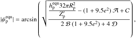 (14)where
![\begin{eqnarray} \nonumber \mathcal{A} & \coloneqq& 4 \varepsilon_{0,i} + e^2 {\Big [}-20 \varepsilon_\mathrm{0,p} + 49 \varepsilon_\mathrm{1,p} + \varepsilon_\mathrm{2,p} {\Big ]} \\ \nonumber \mathcal{B} & \coloneqq& -2 \varepsilon_\mathrm{0,p} + \varepsilon_\mathrm{8,p} + \varepsilon_\mathrm{9,p}\\ \nonumber \mathcal{C} & \coloneqq& 4 \varepsilon_\mathrm{0,p} + e^2 {\Big [}-20 \varepsilon_\mathrm{0,p} + \frac{147}{2} \varepsilon_\mathrm{1,p} + \frac{1}{2} \varepsilon_\mathrm{2,p} - 3\varepsilon_\mathrm{5,p} {\Big ]}\\ \mathcal{D} & \coloneqq& {\Big [} \varepsilon_\mathrm{0,p} - \varepsilon_\mathrm{8,p} {\Big ]}. \end{eqnarray}](/articles/aa/full_html/2011/04/aa15809-10/aa15809-10-eq124.png) (15)For
e ≳ 0.324 Eq. (12)
yields
(15)For
e ≳ 0.324 Eq. (12)
yields  . Thus,
the signs of the phase lags ε0,p,
ε1,p, ε2,p,
ε8,p, and ε9,p make a discrete
jump to + 1. Hence
. Thus,
the signs of the phase lags ε0,p,
ε1,p, ε2,p,
ε8,p, and ε9,p make a discrete
jump to + 1. Hence  and Eq. (14)has no analytic solution.
Moreover, in this case all the terms depending on ψp vanish in
Eq. (11) because
ε0,p = ε8,p and
2ε0,p = ε8,p + ε9,p.
Therefore the concept of maximum or minimum obliquity consistent with a given heating rate
cannot apply. This situation is a direct result of the exclusion of higher order terms in
the second order CPL model and is an important limitation of the
low e-low ψ approximations. If more frequencies were
added, this degeneracy would arise at higher eccentricities.
and Eq. (14)has no analytic solution.
Moreover, in this case all the terms depending on ψp vanish in
Eq. (11) because
ε0,p = ε8,p and
2ε0,p = ε8,p + ε9,p.
Therefore the concept of maximum or minimum obliquity consistent with a given heating rate
cannot apply. This situation is a direct result of the exclusion of higher order terms in
the second order CPL model and is an important limitation of the
low e-low ψ approximations. If more frequencies were
added, this degeneracy would arise at higher eccentricities.
2.3. Equilibrium tide with constant time lag (CTL)
Lec10 extended the model presented by Hut (1981)
to arbitrary eccentricities and obliquities. For convenience and to ease comparison with
the CPL model, we rewrite their equations for the evolution of the orbital parameters as
![\begin{eqnarray} \label{equ:e_Lec} \frac{\mathrm{d}e}{\mathrm{d}t} & =& \ \frac{11 ae}{2 G M_1 M_2} \sum_{i \, \neq \, j}Z_i \left( \cos(\psi_i) \frac{f_4(e)}{\beta^{10}(e)} \frac{\omega_i}{n} -\frac{18}{11} \frac{f_3(e)}{\beta^{13}(e)} \right) \\ \frac{\mathrm{d}a}{\mathrm{d}t} \ &=& \ \frac{2 a^2}{G M_1 M_2} \sum_{i \, \neq \, j} Z_i \left( \cos(\psi_i) \frac{f_2(e)}{\beta^{12}(e)} \frac{\omega_i}{n} - \frac{f_1(e)}{\beta^{15}(e)} \right) \\ \frac{\mathrm{d}\omega_i}{\mathrm{d}t} \ &=& \ \frac{Z_i}{2 M_i r_{\mathrm{g},i}^2 R_i^2 n} \left( 2 \cos(\psi_i) \frac{f_2(e)}{\beta^{12}(e)} - \left[ 1+\cos^2(\psi) \right] \frac{f_5(e)}{\beta^9(e)} \frac{\omega_i}{n} \right) ~~~~~~~~~ \\ \label{equ:psi_LEC} \frac{\mathrm{d}\psi_i}{\mathrm{d}t} \ &=& \ \frac{Z_i \sin(\psi_i)}{2 M_i r_{\mathrm{g},i}^2 R_i^2 n \omega_i}\left( \left[ \cos(\psi_i) - \frac{\xi_i}{ \beta} \right] \frac{f_5(e)}{\beta^9(e)} \frac{\omega_i}{n} - 2 \frac{f_2(e)}{\beta^{12}(e)} \right) \label{equ:psi_LEC} \end{eqnarray}](/articles/aa/full_html/2011/04/aa15809-10/aa15809-10-eq137.png) where
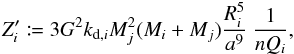
where
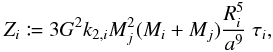 (20)k2,iis
the potential Love number of degree 2 of the ith body, and the extension functions in
e are
(20)k2,iis
the potential Love number of degree 2 of the ith body, and the extension functions in
e are 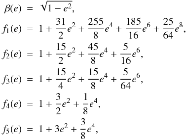 (21)following
the nomenclature of Hut (1981). When
e = 0 all these extensions converge to 1. Furthermore, for
τi = 1/(nQi)
one finds
(21)following
the nomenclature of Hut (1981). When
e = 0 all these extensions converge to 1. Furthermore, for
τi = 1/(nQi)
one finds  .
.
The tidal heating rate in the ith body is given by ![\begin{eqnarray} \label{equ:heat} \nonumber \dot{E}_{\mathrm{tid},i} &= &\ Z_i {\Bigg (} \frac{f_1(e)}{\beta^{15}(e)} - 2 \frac{f_2(e)}{\beta^{12}(e)} \cos(\psi_i) \frac{\omega_i}{n} \\ && + {\Big [} \frac{1+\cos^2(\psi_i)}{2} {\Big ]} \frac{f_5(e)}{\beta^9(e)} \left\{\frac{\omega_i}{n} \right\}^2 {\Bigg )} . \end{eqnarray}](/articles/aa/full_html/2011/04/aa15809-10/aa15809-10-eq143.png) (22)The
equilibrium rotation rate is
(22)The
equilibrium rotation rate is 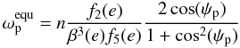 (23)(see
also Levrard et al. 2007; Wisdom 2008), and therefore Eq. (22) can be written as
(23)(see
also Levrard et al. 2007; Wisdom 2008), and therefore Eq. (22) can be written as ![\begin{equation} \label{equ:heat_equ} \dot{E}_{\mathrm{tid},p}^{\mathrm{equ}} = \frac{Z_\mathrm{p}}{\beta^{15}(e)} \left[ f_1(e) - \frac{f_2^2(e)}{f_5(e)} \frac{2 \cos^2(\psi_\mathrm{p})}{1+\cos^2(\psi_\mathrm{p})} \right] \end{equation}](/articles/aa/full_html/2011/04/aa15809-10/aa15809-10-eq145.png) (24)for
a planet in equilibrium rotation. This function of ψp has
minima at ψp = 0° ∨ 180° and maximum at
ψp = 90°. The symmetry of tidal heating around 90°
simply mirrors the fact that a translation between
(ψp,
(24)for
a planet in equilibrium rotation. This function of ψp has
minima at ψp = 0° ∨ 180° and maximum at
ψp = 90°. The symmetry of tidal heating around 90°
simply mirrors the fact that a translation between
(ψp, ) and
(π − ψp,
) and
(π − ψp, ) results in
identical physical states.
) results in
identical physical states.
For a given surface heating rate  of a planet
in equilibrium rotation, Eq. (24) becomes
of a planet
in equilibrium rotation, Eq. (24) becomes
![\begin{equation} \label{equ:tilt_LEC} |\psi_\mathrm{p}^{\mathrm{equ}}| = \arccos\left(\left\{ \left[\displaystyle f_1(e) - \frac{\displaystyle 4 \pi R_\mathrm{p}^2 h_\mathrm{p}^\mathrm{equ} \beta^{15}(e)}{\displaystyle Z_\mathrm{p}} \right]^{-1}\frac{\displaystyle 2 f_2^2(e)}{\displaystyle f_5(e)}-1 \right\}^{-1/2} \right) \end{equation}](/articles/aa/full_html/2011/04/aa15809-10/aa15809-10-eq153.png) (25)for
(25)for
 .
.
2.4. Comparison of CPL and CTL models
Both models converge for a limiting case, namely when both e → 0
and ψ → 0. If we assume that tides have circularized the orbit and
the rotation rate of the planet has been driven close to its equilibrium rotation,
ωp = n in the CPL model1, then the signs of the tidal phase lags become
ε0,i = 0,
ε1,i = −1,
ε2,i = 1,
ε5,i = 1,
ε8,i = −1, and
ε9,i = 1. As an example consider the
differential equation for the evolution of the obliquity. The other equations behave
similarly. For e → 0 and
ψi → 0, Eq. (5) transforms into ![\begin{equation} \label{equ:psi_converge_FM} \frac{\mathrm{d}\psi_i}{\mathrm{d}t} = - \frac{Z'_i \ \psi_i}{2 M_i r_{\mathrm{g},i}^2 R_i^2 n \omega_i} {\Big [} 1+\xi_i {\Big ]} , \end{equation}](/articles/aa/full_html/2011/04/aa15809-10/aa15809-10-eq164.png) (26)while Eq. (19) from the CTL model at first order in
ψ and for e = 0 gives
(26)while Eq. (19) from the CTL model at first order in
ψ and for e = 0 gives ![\begin{equation} \label{equ:psi_converge_LEC} \frac{\mathrm{d}\psi_i}{\mathrm{d}t} = - \frac{Z_i \ \psi_i}{2 M_i r_{\mathrm{g},i}^2 R_i^2 n \omega_i} \left[ 1 + \xi_i \right] \cdot \end{equation}](/articles/aa/full_html/2011/04/aa15809-10/aa15809-10-eq165.png) (27)Equations (26) and (27) coincide for
τi = 1/(nQi),
which is the value of the specific dissipation function for a quasi-circular
pseudo-synchronous planet (see Sect. 3 in Lec10).
(27)Equations (26) and (27) coincide for
τi = 1/(nQi),
which is the value of the specific dissipation function for a quasi-circular
pseudo-synchronous planet (see Sect. 3 in Lec10).
3. Constraints on habitability from obliquity tides
3.1. Tilt erosion
We define the “tilt erosion time” tero as the time required to reduce an initial Earth-like obliquity of 23.5° to 5°. We numerically integrate the two sets of coupled equations from Sects. 2.2 and 2.3, respectively, to derive tero over a wide range of e, a, and Ms. We choose two different planetary masses: an Earth-twin of one Earth mass and a Super-Earth of of 10 Earth masses. Planets are released with initial rotation periods of 1 d orbiting the IHZs around stars with masses up to 1 M⊙.
3.2. Tidal heating from obliquity tides
To calculate the obliquities  and
and
 of a planet we use the adopted
minimum and maximum surface heating rates of 0.04 W/m2 and 2 W/m2,
respectively. Close to the star tidal heating will be ≫ 2 W/m2 even without
heating from obliquity tides, whereas in the outer regions obliquity tides may push the
rates above the 2 W/m2 threshold or not – depending on the actual obliquity.
Further outside, there will be a minimum obliquity necessary to yield
of a planet we use the adopted
minimum and maximum surface heating rates of 0.04 W/m2 and 2 W/m2,
respectively. Close to the star tidal heating will be ≫ 2 W/m2 even without
heating from obliquity tides, whereas in the outer regions obliquity tides may push the
rates above the 2 W/m2 threshold or not – depending on the actual obliquity.
Further outside, there will be a minimum obliquity necessary to yield
 W/m2. We should
bear in mind that these key heating rates of 0.04 W/m2 and 2 W/m2
are empirical examples taken from two special cases the Solar System. Depending on a
planet’s structure, composition, and age these thresholds may vary significantly. In
general, the connection between surface heating rates and geologic activity is still
subject to fundamental debate.
W/m2. We should
bear in mind that these key heating rates of 0.04 W/m2 and 2 W/m2
are empirical examples taken from two special cases the Solar System. Depending on a
planet’s structure, composition, and age these thresholds may vary significantly. In
general, the connection between surface heating rates and geologic activity is still
subject to fundamental debate.
3.3. Tidal locking vs. equilibrium rotation
A widely spread misapprehension is that a tidally locked body permanently turns one side to its host (e.g. in Neron de Surgy & Laskar 1997; Joshi et al. 1997; Grießmeier et al. 2004; Khodachenko et al. 2007). Various other studies only include the impact of eccentricity on tidal locking, neglecting the contribution from obliquity (Goldreich & Soter 1966; Goldreich 1966; Eggleton et al. 1998; Trilling 2000; Showman & Guillot 2002; Dobbs-Dixon et al. 2004; Selsis et al. 2007; Barnes et al. 2008). As long as “tidal locking” denotes only the state of dωp/dt = 0, the actual equilibrium rotation period, as predicted by the CTL model of Lec10, may differ from the orbital period, namely when e ≠ 0 and/or ψp ≠ 0. Only if “tidal locking” depicts the recession of tidal processes in general, when e = 0 and ψp = 0 in Lec10’s model, then ωp = n. As given by Eq. (23), one side of the planet is permanently orientated towards the star if both e = 0 and ψ = 0 [2]. In this case, habitability of a planet can potentially be ruled out when the planet’s atmosphere freezes out on the dark side and/or evaporates on the bright side (Joshi et al. 1997). As long as e and ψp are not eroded, however, the planet can be prevented from an ωp = n locking. In the CPL model, however, the equilibrium rotation state is not a function of ψp, thus “tidal locking”, denoting dωp/dt = 0, indeed can occur for ψp ≠ 0.
In addition to atmospheric instabilities arising from ωp = n, slow rotation may result in small intrinsic magnetic moments of the planet. This may result in little or no magnetospheric protection of planetary atmospheres from dense flows of coronal mass ejection plasma of the host star (Khodachenko et al. 2007) (but see also Gomez-Perez et al. 2010; Gregory 2011, who make counterpoints). Again, since obliquities can prevent a synchronous rotation of the planet with the orbit, its magnetic shield can be maintained. An example of equilibrium rotation rates is shown in Barnes et al. (2010a). Below, we apply the CPL and the CTL models to the Super-Earth Gl581 d and explore its tidal equilibrium period as a function of e and ψp.
3.4. Compatibility with the insolation habitable zone
Our constraints on habitability from obliquity tides are embedded in the IHZ as presented by Barnes et al. (2008), who enhanced the model of Selsis et al. (2007) to arbitrary eccentricities (Williams & Pollard 2002).
The first forms of life on Earth required between 0.3 and 1.8 Gyr to emerge (Gaidos et al. 2005). During this period, before the
so-called Great Oxidation Event ≈2.5 Gyr ago (Anbar
et al. 2007), microorganisms may have played a major role in the evolution of
Earth’s atmosphere (Kasting & Siefert
2002), probably enriching it with CH4 (methane) and CO2
(carbon dioxide). On geological times it was only recently that life conquered the land,
about 450 Myr ago in the Ordovician (Kenrick &
Crane 1997; Kenrick 2003). Therefore it is
reasonable to assume that a planet needs to provide habitable conditions for at least
1 Gyr for life to imprint its spectroscopic signatures in the planet’s atmosphere (Seager et al. 2002; Jones & Sleep 2010) or to leave photometrically detectable traces on the
planet’s surface (Fujii et al. 2010). This is
relevant from an observational point of view since the spectra of Earth-like planets will
be accessible with upcoming space-based missions such as Darwin (Ollivier & Léger 2006; Léger
& Herbst 2007) and the Terrestrial Planet Finder (Kaltenegger et al. 2010a). For this reason, when our two test objects
in the IHZ show either tero ≪ 1 Gyr or
 W/m2, constraints on
the habitability of the planet will be appreciable.
W/m2, constraints on
the habitability of the planet will be appreciable.
4. Results
4.1. Time scales for tilt erosion
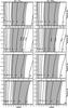 |
Fig. 1 Tilt erosion times for FM08. The IHZ is shaded in gray, contours of constant tero are labeled in units of log (tero/yr). Error estimates for Qp are shown for the 0.25 M⊙ star. |
We plot tero for an Earth twin and a 10-Earth-mass planet orbiting a 0.1, 0.25, 0.5, and 0.75 M⊙ star in Fig. 1 (CPL) and Fig. 2 (CTL). In Figs. 3 and 4 we plot tero for the two planets over a range of stellar masses and initial semi-major axes, for the two cases of initial eccentricities e = 0.01 and e = 0.5. We also include a few examples for different choices for Qp. The IHZs are shaded in grey. tero increases with increasing initial distance from the star as well as with decreasing initial eccentricity. In eccentric orbits at short orbital distances the obliquity is eroded most rapidly.
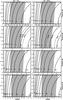 |
Fig. 2 Tilt erosion times for Lec10. The IHZ is shaded in gray, contours of constant tero are labeled in units of log (tero/yr). Error estimates for Qp are shown for the 0.25 M⊙ star. |
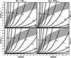 |
Fig. 3 Tilt erosion times for FM08. The IHZ is shaded in gray and the contours of constant tilt erosion times are labeled in units of log (tero/yr). |
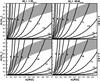 |
Fig. 4 Tilt erosion times for Lec10. The IHZ is shaded in gray and the contours of constant tilt erosion times are labeled in units of log (tero/yr). |
For the FM08 model in Fig. 1, we see that tero ≲ 0.1 Gyr for Ms ≲ 0.25 M⊙ for both planets in the IHZ. For Ms = 0.75 M⊙ obliquities resist erosion for ≳ 0.1 Gyr throughout the IHZ. Although we do not show the corresponding figures, we find that if the star has a mass ≳ 1 M⊙ the IHZ is completely covered with tero > 10 Gyr – for all the three reasonable Q values of both planets.
The calculations following Lec10 (Fig. 2) yield qualitatively similar results for small eccentricities. However, for e ≳ 0.3 their mismatch is of the same order of magnitude as the uncertainty in the tidal dissipation function Q (see the 0.25 M⊙ row). For these high eccentricities, the CTL model of Lec10 predicts significantly smaller tilt erosion times, where the discrepancy is also stronger for lower-mass stars.
A comparison of Figs. 1 and 2 at e = 0 shows that, for a given combination of planetary and stellar mass, the contours for tero = 107 yr meet the abscissa at almost the same semi-major axis. For regions closer to the star, tilt erosion times provided by the CTL model are shorter. Farther outside, however, the CPL model yields smaller values for tero at e = 0. On the one hand, these discrepancies follow from the different forms of the differential equations – remember that, although e = 0, the initial obliquity ψp = 23.5° and thus the CPL and the CTL do not converge as demonstrated in Eqs. (26)and (27)for e = 0 ∧ ψp = 0. On the other hand, the incompatible values for Qp and τp (see Sect. 2.1.2) lead to different evolutionary speeds in the two models.
The projection of tero onto the Ms-a plane based on the FM08 model is shown in Fig. 3. For the Earth twin in the e = 0.01 case (upper left panel) we find that the complete IHZ is covered by tero > 1 Gyr as long as Ms ≳ 0.8 M⊙, where the inner border of the IHZ is at roughly 0.4 AU. For an eccentricity of 0.5 (lower left panel) the Earth-sized planet requires an Ms ≳ 0.85 M⊙ host star, thus a minimum semi-major axis of 0.5 AU, for tilt erosion times larger than 1 Gyr throughout the IHZ. The larger moment of inertia of the 10 MEarth Super-Earth (panels in the right column) assures that the initial obliquity of 23.5° is washed out on timescales > 1 Gyr even for slightly tighter orbits in the IHZ and somewhat lower-mass stars at both eccentricities. Comparing the upper and lower panel rows, corresponding to e = 0.01 at the top and e = 0.5 at the bottom, one sees that higher eccentricities tend to erode the spin faster by a factor of 3.
The higher order terms of e in the equations of Lec10 produce a large discrepancy in tero between e = 0.01 (upper panel) and e = 0.5 (lower panel) in Fig. 4. While the results for e = 0.01 almost coincide with those of the FM08 model, Lec10 predicts much more rapid tilt erosion for e = 0.5. The magnification of tidal effects at high eccentricities is due to the plummet of the mean orbital distance in eccentric orbits and is enhanced by the steep dependency of tidal effects on a (Wisdom 2008; Leconte et al. 2010). This behavior at high eccentricities is due to the slow convergence of elliptical expansion series and has been studied in detail by Cottereau et al. (2010). For the lower left panel, where e = 0.5 for the Earth-sized planet, an Ms ≳ 0.9 M⊙ host is necessary for tero > 1 Gyr over the whole IHZ, with the inner border at about 0.55 AU. Again, the Super-Earth is slightly more resistive to tilt erosion. A compelling outcome of this visualization is that the Lec10 model predicts tero < 10 Gyr for an Earth-mass planet at the inner edge of the IHZ of a 1 M⊙ star if the initial eccentricity is larger than 0.5.
4.2. Tidal heating from obliquity tides
In Fig. 5 we plot
 and
and
 as a
function of a and e for an Earth-mass planet orbiting
stars with four different masses, as above. Results for the
10 MEarth terrestrial planet are not shown because they
are very similar. The left column shows the results for the CPL model and the right column
the CTL model. The white space in the left panels is due to the ambiguity of Eq. (14)as explained at the end of Sect. 2.2. Red zones indicate that even for the case of
as a
function of a and e for an Earth-mass planet orbiting
stars with four different masses, as above. Results for the
10 MEarth terrestrial planet are not shown because they
are very similar. The left column shows the results for the CPL model and the right column
the CTL model. The white space in the left panels is due to the ambiguity of Eq. (14)as explained at the end of Sect. 2.2. Red zones indicate that even for the case of
 , tidal surface
heating rates are
, tidal surface
heating rates are  . Starting from the
left in a certain panel, the contours illustrate a maximum obliquity of
1°,20°,30°,40°,50°,60°,70°,80°, and 89°, all of which produce
. Starting from the
left in a certain panel, the contours illustrate a maximum obliquity of
1°,20°,30°,40°,50°,60°,70°,80°, and 89°, all of which produce
 at their
respective localization in the a-e plane. Green in
Fig. 5 depicts a region where neither any obliquity
produces tidal surface heating rates > 2 W/m2 nor any minimum
obliquity is required to yield tidal surface heating rates
> 0.04 W/m2. The 9-tuple of contour lines for
refers to
obliquities of 1°,20°,...,80°, and 89° providing
at their
respective localization in the a-e plane. Green in
Fig. 5 depicts a region where neither any obliquity
produces tidal surface heating rates > 2 W/m2 nor any minimum
obliquity is required to yield tidal surface heating rates
> 0.04 W/m2. The 9-tuple of contour lines for
refers to
obliquities of 1°,20°,...,80°, and 89° providing
 at their
respective localization. Smaller obliquities lead to less tidal heating. In the blue zone
finally, not even a planet with a rotational axis perpendicular to the orbital plane
normal, e.g. ψp = 90°, yields
at their
respective localization. Smaller obliquities lead to less tidal heating. In the blue zone
finally, not even a planet with a rotational axis perpendicular to the orbital plane
normal, e.g. ψp = 90°, yields
 .
.
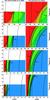 |
Fig. 5 Obliquity thresholds ψmax and
ψmin as explained in the text. For each 9-tuple of
contours the lines indicate 1°,20°,30°,...,70°,80°, and 89°. The
IHZ is indicated with dashed lines. In the red zone,
|

Both models predict that Earth-like planets in the inner IHZ of stars with masses
≈ 0.1 M⊙ are subject to intense tidal heating, while
tidal heating in the outer zone of the IHZ is more moderate for the CPL model. With
increasing stellar mass the IHZ is shifted to wider orbits for both models, whereas the
green stripe of moderate tidal heating is located at roughly the same position in all the
8 panels of Fig. 5. This is due to the weak
sensitivity of  on
Ms compared to the sensitivity on a. The
IHZ of a 0.25 M⊙ star nicely covers the zone with moderate
tidal heating. In this overlap, adequate stellar insolation meets tolerable tidal heating
rates. Only highly eccentric orbits at the inner IHZ are subject to extreme tidal heating,
as shown in the right column for the CTL model. Terrestrial planets in the IHZ of
0.5 M⊙ stars do not undergo intense tidal heating. Only at
the inner border of the IHZ
on
Ms compared to the sensitivity on a. The
IHZ of a 0.25 M⊙ star nicely covers the zone with moderate
tidal heating. In this overlap, adequate stellar insolation meets tolerable tidal heating
rates. Only highly eccentric orbits at the inner IHZ are subject to extreme tidal heating,
as shown in the right column for the CTL model. Terrestrial planets in the IHZ of
0.5 M⊙ stars do not undergo intense tidal heating. Only at
the inner border of the IHZ  for high
obliquities, while at the outer regions tidal heating rates are of order
10 mW/m2 and smaller even for ψp = 90°.
For terrestrial planets in the IHZ of stars with masses
≳ 0.75 M⊙, both models indicate that tidal heating has
negligible impact on the planet’s energy budget and that it does not induce constraints on
the planet’s habitability.
for high
obliquities, while at the outer regions tidal heating rates are of order
10 mW/m2 and smaller even for ψp = 90°.
For terrestrial planets in the IHZ of stars with masses
≳ 0.75 M⊙, both models indicate that tidal heating has
negligible impact on the planet’s energy budget and that it does not induce constraints on
the planet’s habitability.
4.3. Gl581 d and g as examples
Gl581 d is an
Mp ≈ 5.6 MEarth
Super-Earth, grazing the outer rim of the IHZ of its
Ms ≈ 0.29 M⊙ host star
(Bonfils et al. 2005b; Selsis et al. 2007; von Bloh et al.
2007; Beust et al. 2008; Barnes et al. 2009; Mayor et al. 2009; Wordsworth et al.
2010; Vogt et al. 2011). The apoastron is
situated outside the IHZ whereas the periastron is located inside. While the solar
constant, i.e. the solar energy flux per time and area on the Earth’s surface, is about
1000 W/m2 when the Sun is in the zenith3, the stellar incident flux on Gl581 d averaged over an orbit (Williams & Pollard 2002) is
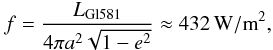 (28)with the luminosity
of the host star
LGl581 = 0.013 L⊙ (Bonfils et al. 2005a; Mayor et al. 2009). If the absorbed stellar flux per unit area is larger than
≈ 300 W/m2, runaway greenhouse effects may turn a terrestrial planet
uninhabitable (Zahnle et al. 2007; Selsis et al. 2007, and references therein). Thus, the
maximum bond albedo for Gl581 d compatible with this habitability criterion is
300/432 ≈ 0.7. A recent study on atmospheric constraints on the habitability of
Gl581 d is given by von Paris et al. (2010).
(28)with the luminosity
of the host star
LGl581 = 0.013 L⊙ (Bonfils et al. 2005a; Mayor et al. 2009). If the absorbed stellar flux per unit area is larger than
≈ 300 W/m2, runaway greenhouse effects may turn a terrestrial planet
uninhabitable (Zahnle et al. 2007; Selsis et al. 2007, and references therein). Thus, the
maximum bond albedo for Gl581 d compatible with this habitability criterion is
300/432 ≈ 0.7. A recent study on atmospheric constraints on the habitability of
Gl581 d is given by von Paris et al. (2010).
 |
Fig. 6 Left: evolution of the putative rotation period for Gl581 d for both models, FM08 and Lec10. The initial period was taken to be analog to the Earth’s current day. The filled circle at ≈ 25.3 Myr on the Lec10 track indicates ωp/n ≲ 6.13, thus from then on dψp/dt < 0, as given by Eq. (29). Right: evolution of a putative initial Earth-analog obliquity for Gl581 d for both models, FM08 and Lec10. |
If confirmed, the recently detected planet candidate Gl581 g (Vogt et al. 2011; Anglada-Escudé 2010) is located more suitably in the IHZ of Gl581, but it does not show a significant eccentricity. Since eccentricity has a crucial impact on a planet’s orbital evolution, we choose Gl581 d as an example to study the change of its spin orientation and period as well as its current tidal heating. An analysis of tidal heating in Gl581 g is given at the end if this section. Since we take the parameters for Gl581 d from Mayor et al. (2009) and the parameters for planet g from Vogt et al. (2011), our model for the two tidal evolutions need not necessarily be consistent.
For the tidal evolution of Gl581 d, a comparison between the FM08 and the Lec10 models is
applied where it is reasonable. As initial obliquities we take 23.5° for the planet and 0°
for the star, the initial rotation periods are 1 d for the planet and 94.2 d for the star
(Vogt et al. 2011). The remaining physical
quantities of the host star and the two planets are assumed as explained in Sect. 2.1.2. For both models we find insignificant decreases in
e during the lifetime of the system, which has been estimated to
≳ 2 Gyr (Bonfils et al. 2005b) and ≈ 4.3 Gyr
(Vogt et al. 2011). In the long term, FM08’s
model predicts a negligible increase of a, while Lec10’s model yields an
insignificant decrease. As shown in the left panel of Fig. 6, both models predict a steady increase of the rotation period of Gl581 d. For
the model of Lec10, the numeric solution for the equilibrium rotation period of
Pequ ≈ 35 d can also be calculated analytically with
Eq. (23), using the observed
eccentricity e = 0.38 ( ± 0.09) and assuming that the spin
axis is co-aligned with the orbit normal, ψp = 0°. In
the right panel of Fig. 6, both models predict d’s
obliquity has been eroded over the course of the system’s evolution, assuming no
perturbations from other bodies. At an age of ≲ 0.1 Gyr, tidal processes would have
pushed an Earth-like initial obliquity to zero and the rotation is most likely caught in
its equilibrium state. In both models the obliquity of the planet first increases to
≈ 51° before it is finally eroded. The reason for the change in the algebraic sign of
dψp/dt is found, when one sets
dψp/dt > 0. Considering that
ξp ≪ 1 for Gl581 d,
dψp/dt > 0 in Eq. (19)is equivalent to  (29)For
ψp = 51° we find
ωp/n ≳ 6.13. After about 25.3 Myr
in our simulations with the model of Lec10, the rotation has slowed down to
ωp/n ≲ 6.13 (see left panel in
Fig. 6), thus
dψp/dt < 0. For the rest of
the evolution dψp/dt < 0 since
the orbital period keeps increasing until it reaches the equilibrium state. Comparing both
panels of Fig. 6, we find that the time scale for the
relaxation of the obliquity is longer than the time scale for the restoration of the
equilibrium rotation period. This behavior has recently been explained by Correia (2009).
(29)For
ψp = 51° we find
ωp/n ≳ 6.13. After about 25.3 Myr
in our simulations with the model of Lec10, the rotation has slowed down to
ωp/n ≲ 6.13 (see left panel in
Fig. 6), thus
dψp/dt < 0. For the rest of
the evolution dψp/dt < 0 since
the orbital period keeps increasing until it reaches the equilibrium state. Comparing both
panels of Fig. 6, we find that the time scale for the
relaxation of the obliquity is longer than the time scale for the restoration of the
equilibrium rotation period. This behavior has recently been explained by Correia (2009).
As given by Eq. (23) from the CTL theory and as explained in Sect. 3.3, the equilibrium rotation period is also a function of e and ψp. We calculate the equilibrium rotation period Pequ as a function of the obliquity ψp for a set of eccentricities (Fig. 7). The most likely value of Pequ ≈ 35 d, corresponding to e = 0.38 and ψp ≲ 40°, can be inferred from the gray line in Fig. 7 for e = 0.4. Since the observed orbital period of Gl581 d is about 68 d, Fig. 7 shows that Gl581 d does not permanently turn one hemisphere towards its host star, except for the cases of ψp ≈ 74° ∨ 106°. And even then the obliquity is so large that most of the surface cycles in and out of starlight over an orbit.
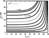 |
Fig. 7 Equilibrium rotation period of Gl581 d as a function of obliquity for various eccentricities, following the model of Lec10. The gray line corresponds to e = 0.4, close to the observed eccentricity of e = 0.38 ( ± 0.09) (Mayor et al. 2009). The observed orbital period is indicated with a dotted line. |
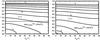 |
Fig. 8 Tidal surface heating rates, including eccentricity and obliquity heating, on Gl581 d (left panel) and Gl581 g (right panel) following the model of Lec10 as a projection on the parameter plane spanned by obliquity ψp and eccentricity e. Equilibrium rotation of the planets is assumed. The observed eccentricity of 0.38 ( ± 0.09) for Gl581 d (Mayor et al. 2009) is indicated with a dashed line, while the eccentricity of Gl581 g is compatible with 0. Depending on obliquity, tidal surface heating rates on Gl581 d vary between roughly 2 and 15 mW/m2, while on planet candidate g they are < 150 mW/m2 as long as e ≲ 0.3. |
We have done the same calculations of the tidal evolution for Gl581 g, assuming a slight orbital eccentricity of 0.01 and a mass of 3.1 MEarth, corresponding to its projected minimum mass (Vogt et al. 2011). In brief, we find an evolutionary scenario similar to that of planet d but on a considerably shorter timescale. After ≈ 20 Myr both tidal models predict a locking in equilibrium rotation at almost exactly the orbital period of ≈ 36.56 d. The evolution of ψp for planet g looks almost the same as for planet d, except that the obliquity is eroded about a factor of 5 faster in FM08’s model and about a factor of 3 faster in the model of Lec10, due to the smaller planetary mass and semi-major axis of planet g.
In Fig. 8 we present the tidal surface heating rates, including obliquity heating, of Gl581 d and g as a function of their putative obliquity. Since these planets encounter considerable interactions with the remaining four planets of the system, all orbits might be significantly tilted against each other (see Sect. 1.2). Thus, the obliquities ψp of the planets might be significant. Between spin-orbit alignment (ψp = 0°) and a planetary spin axis perpendicular to the orbital plane (ψp = 90°) tidal surface heating rates on Gl581 d (left panel in Fig. 8) range from roughly 2 to about 15 mW/m2, given that e = 0.38 (±0.09). As a comparison, we show the tidal surface heating of the potentially habitable planet Gl581 g in the right panel of Fig. 8. Measurements by Vogt et al. (2011) indicate that the eccentricity of Gl581 g is small if not zero. As long as its eccentricity is < 0.3 we find tidal heating on Gl581 g to be ≲150 mW/m2. Only if the planet’s eccentricity has been ≳0.5 in the history of the system, high obliquities could have produced tidal surface heating rates of ≈1 W/m2 (upper half in the right panel of Fig. 8).
The eccentricities of the planets around Gl581 could be subject to fluctuations. In their history, their values might have been significantly larger than their current values. For reasonable eccentricities < 0.7 of Gl581 d, we find that tidal surface heating rates on this planet have always been smaller than 1 W/m2 if the planet’s semi-major axes has never been significantly smaller than its current value. On planet g tidal heating will be negligible if its eccentricity turns out to be < 0.3.
5. Discussion
Our results for tilt erosion, tidal heating, and equilibrium rotation picture scenarios for atmospheric scientists and geophysicists. For low planetary obliquities, atmospheres of planets at the outer border of the IHZ can be subject to freeze out at the planet’s poles (priv. comm. with Franck Selsis). Moreover, ψp → 0 weakens the seasonal temperature contrast at a given location on the planetary surface but strengthens the temperature contrast as a function of latitude (see Sect. 1.1). Given the mass and the age of a star, as well as the orbital parameters of the planet, our estimates of the tilt erosion time scales indicate whether a significant obliquity of the planet is likely. Our choice of 5° as the final obliquity for the computation of tero is somewhat arbitrary but the time for ψp to decline from 5° to 0.5° and even to 0.05° is usually much smaller than tero as we use it (see right panel in Fig. 6). In any case, if low obliquities constrain the habitability of exoplanets, then the respective effects are likely to occur for ψp of the order of a few degrees and far before it has reached 0.
The spin angular momentum history of a planet, i.e. the evolution of obliquity and rotation rate, is a crucial feature of planetary climate. We encourage climate modelers to consider the diversity of atmospheres that are possible within the constraints outlined above.
Our exploration of tidal heating will be relevant for structural evolution models of terrestrial planets. Moreover, the tidal response is a function of the internal structure, hence a natural feedback mechanism exists between the two. The structure and cooling of Super-Earths have recently been explored in the literature (e.g. by Sleep 2000; Valencia et al. 2007; O’Neill & Lenardic 2007; Kite et al. 2009; Stamenkovic et al. 2009; Plesa & Breuer 2009), but a consensus has yet to emerge. On the one hand, the heat flow out of the interior should scale as the ratio of volume to the surface area, i.e. ∝ Ri. This relationship just assumes that larger planets have more radiogenic isotopes. Therefore large terrestrial planets seem more likely to have mobile lids than the Earth. On the other hand, larger planets have stronger gravitational fields and hence planets may fuse together due to the higher overburden pressure. Therefore large terrestrial planets seem more likely to have stagnant lids than the Earth. As if the story was not complicated enough already, none of those studies considered any potential tidal heating. Hence the issue for planets in the IHZ of LMSs is further complicated, but at least appears ripe for observational constraints: As recently shown by Kaltenegger et al. (2010b), acute volcanism on Earth-like planets will be detectable with the James Webb Space Telescope. Our calculations suggest that such worlds orbiting ≲ 0.25 M⊙ stars orbiting closer than 0.1 AU will present promising targets.
Tidal heating rates, as given by the models of Lec10 and FM08, are a function of
e and ψp, amongst others. For Gl581 d we find
 for its current
eccentricity. This is in line with the value of 0.01 W/m2 estimated by Barnes et al. (2009), who neglected the planet’s
obliquity. We also explore
for its current
eccentricity. This is in line with the value of 0.01 W/m2 estimated by Barnes et al. (2009), who neglected the planet’s
obliquity. We also explore  as a function
of the planet’s eccentricity and find that tidal heating is unlikely to have constrained the
habitability of the planet since
as a function
of the planet’s eccentricity and find that tidal heating is unlikely to have constrained the
habitability of the planet since  as long as
e < 0.7. Tidal heating on the exoplanet candidate Gl581 g,
which would orbit its host star in the IHZ, is ≲ 150 mW/m2 as long as its
eccentricity is smaller than 0.3.
as long as
e < 0.7. Tidal heating on the exoplanet candidate Gl581 g,
which would orbit its host star in the IHZ, is ≲ 150 mW/m2 as long as its
eccentricity is smaller than 0.3.
Selsis et al. (2007) approximated the rotational
relaxation time of the planet to be 10 Myr, concluding that the planet has one permanent day
side and night side. Indeed, with the revised value of
e = 0.38 ( ± 0.09) (Mayor et al.
2009) we find that the tidal equilibrium rotation occurs after approximately 80 Myr
(Lec10)–90 Myr (FM). However, the equilibrium rotation period of the planet, as calculated
with Lec10’s ansatz, turns out to be  . Correia et al. (2008) have approached the issue of equilibrium rotation of
terrestrial planets for low eccentricities and obliquities. For Gl581 d they found
. Correia et al. (2008) have approached the issue of equilibrium rotation of
terrestrial planets for low eccentricities and obliquities. For Gl581 d they found
 .
.
If the eccentricity of Gl581 g turns out to be 0 and if this state was stable at least over the recent 1 Myr, then tides have driven this planet into an equilibrium rotation state, where both ψp = 0 and e = 0. Due to the smaller planetary mass and semi-major axis, as compared to planet d, Gl581 g is driven into its equilibrium state faster by a factor between 3 (FM08) and 5 (Lec10) in tero.
The semantics of the terms “tidal locking” and “synchronous rotation” carry the risk to cause confusion. Wittgenstein (1953) has pointed out that the meaning of a word is given by its usage in the language (see Sects. 30, 43, and 432 therein). However, “tidal locking” and “synchronous rotation” are used ambiguously in the literature (see Sect. 3.3), thus their meanings remain diffuse. While some authors simply refer to “tidal locking” as the state where a planet permanently turns one hemisphere towards its host star, others use it in a more general sense of tidal equilibrium rotation. Furthermore, the term “pseudo-synchronous rotation” appears, depicting dωp/dt = 0 while ωp ≠ n. We caution that in the CTL model of Lec10 tidal processes drive the planetary rotation period towards the orbital period only if e = 0 and ψp = 0. If a planet with e ≠ 0 or ψp ≠ 0 is said to be tidally locked, then it is clear that tidal locking does not depict the state of the planet turning one hemisphere permanently to its star. However, for certain combinations of e ≠ 0 and ψp ≠ 0 the equilibrium rotation period can yet be equal to the orbital period (see Fig. 7 for Gl581 d, where ωp = n if ψp ≈ 74° ∨ 106°). And in general, the rotation period of the planet will not be synchronized with respect to its orbit, if ‘synchronous’ here means “equal” or “identical”. In general, we call dωp/dt = 0 simply the state of “rotational equilibrium”. When rotational equilibrium meets ωp ≠ n, we call this constellation “pseudo-synchronous”. “Tidal locking” is used when there is no more transfer of angular momentum over the course of one orbit, i.e. e = 0, ψp = 0, and ωp = n. Strictly speaking, a body with e ≠ 0 or ψp ≠ 0 cannot be tidally locked because e and ψp evolve with time.
Uncertainties in our calculations arise from the assumption of a constant tidal dissipation in the planets, parametrized by the tidal dissipation factor Q or τ. For one thing, merging all the geophysical effects such as composition, viscosity, temperature distribution, and pressure in one parameter unquestionably is an oversimplification. In addition, it is unknown how Q depends on the respective tidal frequency. Although on Earth Q is constant over a a wide range of frequencies, the behavior will be different for different objects. The Q value of terrestrial exoplanets remains to be estimated, either by observational constraints or theory. For another thing, whatever Q value will turn out to describe terrestrial planets most reasonably, it will be a function of time due to the structural and rheological evolution of the planet.
Our results need to be considered against the background of further gravitational processes, such as the entourage of massive moons, the Kozai mechanism, Cassini states, planet-planet scattering, and inhomogeneities in the structure of the invoked bodies. These states and processes will add to – and eventually counteract – the tidal evolution. In those cases, significant obliquities could be maintained on time scales much larger or shorter than we present here.
6. Conclusions
Tidal processes raise severe constraints on the habitability of terrestrial planets in the IHZ of LMSs. First, tidal erosion of the obliquities, i.e. “tilt erosion”, of such planets occurs much faster than life emerged on Earth. Planets with masses ≲ 10 MEarth orbiting ≲ 0.25 M⊙ stars in the IHZ lose initial Earth-like spins of 23.5° within less than 0.1 Gyr, typically much faster. In order to cover the complete IHZ with tero > 1 Gyr at high eccentricities, stellar masses ≳ 0.9 M⊙ are required. For terrestrial planets formed in highly eccentric orbits inside the IHZ, tilt erosion can occur within 10 Gyr up to stellar masses of 1 M⊙.
Second, tidal heating of Earth-like planets in the IHZ of stars with ≲ 0.25 M⊙ is significant. Depending on the body’s obliquity, orbital semi-major axis, eccentricity, and its structural composition, a terrestrial planet in the IHZ of a ≲ 0.25 M⊙ host star can undergo intense tidal heating with tidal surface heating rates ≫ 1 W/m2. We find tidal surface heating rates of 2 mW/m2 to 15 mW/m2, depending on ψp, for the Super-Earth candidate Gl581 d and < 150 mW/m2 for Gl581 g. Simulations of coupled orbital-structural evolution of Earth-like planets are necessary to further explore the effect of tidal heating on habitability.
Third, the tidal equilibrium rotation period provided by Lec10 is a function of the
planet’s eccentricity and its obliquity. In general, as long as the planet maintains a
significant obliquity or eccentricity, its rotational equilibrium period will not match the
orbital period. As an example, we deduce the equilibrium rotation period of the extrasolar
Super-Earth Gl581 d to be around 35 d. With an orbital period of roughly 68 d, this means
 . The model of FM08 neglects the
impact of obliquity on the equilibrium rotation state.
. The model of FM08 neglects the
impact of obliquity on the equilibrium rotation state.
For low eccentricities (e ≲ 0.3) and low obliquities (ψp ≲ a few degrees), the CPL model of FM08 and the CTL model of Lec10 mathematically converge. In our calculations of tero (Sect. 4) they provide similar results in the low-eccentricity regime. Since the model of Lec10 considers higher terms in e, tidal processes in the moderate and high eccentricity regime occur on significantly shorter time scales than predicted by FM08. Hence, tidal heating computed with Lec10 is also more intense.
The possible detection of exomoons via transit photometry (Sartoretti & Schneider 1999), the Rossiter-McLaughlin effect (Simon et al. 2010), planet-moon eclipses (Cabrera & Schneider 2007), and transit timing and duration variations (Szabó et al. 2006; Kipping 2009) as well as the empirical constraint of the oblateness of a transiting planet (Carter & Winn 2010a,b), are first steps towards the measurement of the obliquity of exoplanets. All these observational effects are only accessible for transiting planets. Since obliquity determines atmospheric conditions as well as the amount of tidal heating and the equilibrium rotation period, it will be indispensable to verify ψp for planets in the IHZ around their host stars to assess their habitability. Thus, transiting planets are the most promising targets for a comprehensive appraisal of an extrasolar habitat.
Recall Eq. (23) and see that
also
depends on ψp in the CTL model.
Acknowledgments
Our sincere thanks go to Brian Jackson for lively conversations about tidal processes. Virtual discussions with Sylvio Ferraz-Mello have been a valuable stimulation to this study. We appreciate discussions with D. Breuer, H. Rauer, F. Sohl, H. Hussmann, and T. Spohn on a preliminary version of the manuscript. Thanks to the comments of the referee and the editor the understandability of this paper has been significantly improved. This study has benefited from inspirations during the AbGradCon2010 in Tällberg, Sweden. For the most time of the paper processing, R. Heller was supported by a PhD scholarship of the DFG Graduiertenkolleg 1351 “Extrasolar Planets and their Host Stars” at the Hamburger Sternwarte. The research leading to these results has received funding from the European Research Council under the European Community’s Seventh Framework Programme (FP7/2007-2013 Grant Agreement no. 247060). R. Barnes acknowledges funding from NASA Astrobiology Institute’s Virtual Planetary Laboratory lead team, supported by NASA under Cooperative Agreement No. NNH05ZDA001C. R. This research has made use of NASA’s Astrophysics Data System Bibliographic Services.
References
- Agnor, C. B., Canup, R. M., & Levison, H. F. 1999, Icarus, 142, 219 [NASA ADS] [CrossRef] [Google Scholar]
- Anbar, A. D., Duan, Y., Lyons, T. W., et al. 2007, Science, 317, 1903 [NASA ADS] [CrossRef] [PubMed] [Google Scholar]
- Anglada-Escudé, G. 2010, ApJL, Submitted [arXiv:1011.0186] [Google Scholar]
- Barnes, R., Raymond, S. N., Jackson, B., & Greenberg, R. 2008, Astrobiology, 8, 557 [NASA ADS] [CrossRef] [PubMed] [Google Scholar]
- Barnes, R., Jackson, B., Greenberg, R., & Raymond, S. N. 2009, ApJ, 700, L30 [NASA ADS] [CrossRef] [Google Scholar]
- Barnes, R., Jackson, B., Greenberg, R., Raymond, S. N., & Heller, R. 2010a, in Pathways Towards Habitable Planets, ed. V. Coudé du Foresto, D. M. Gelino, & I. Ribas, ASP Conf. Ser., 430, 133 [Google Scholar]
- Barnes, R., Jackson, B., Heller, R., Greenberg, R., & Raymond, S. N. 2010b, LPI Contributions, 1538, 5595 [NASA ADS] [Google Scholar]
- Beust, H., Bonfils, X., Delfosse, X., & Udry, S. 2008, A&A, 479, 277 [NASA ADS] [CrossRef] [EDP Sciences] [Google Scholar]
- Bond, J. C., O’Brien, D. P., & Lauretta, D. S. 2010, ApJ, 715, 1050 [NASA ADS] [CrossRef] [Google Scholar]
- Bonfils, X., Delfosse, X., Udry, S., et al. 2005a, A&A, 442, 635 [NASA ADS] [CrossRef] [EDP Sciences] [Google Scholar]
- Bonfils, X., Forveille, T., Delfosse, X., et al. 2005b, A&A, 443, L15 [NASA ADS] [CrossRef] [EDP Sciences] [Google Scholar]
- Cabrera, J., & Schneider, J. 2007, in Transiting Extrapolar Planets Workshop, ed. C. Afonso, D. Weldrake, & T. Henning, ASP Conf. Ser., 366, 242 [Google Scholar]
- Carter, J. A. & Winn, J. N. 2010a, ApJ, 709, 1219 [NASA ADS] [CrossRef] [Google Scholar]
- Carter, J. A., & Winn, J. N. 2010b, ApJ, 716, 850 [NASA ADS] [CrossRef] [Google Scholar]
- Chambers, J. E. 2001, Icarus, 152, 205 [NASA ADS] [CrossRef] [Google Scholar]
- Correia, A. C. M. 2009, ApJ, 704, L1 [NASA ADS] [CrossRef] [Google Scholar]
- Correia, A. C. M., Levrard, B., & Laskar, J. 2008, A&A, 488, L63 [NASA ADS] [CrossRef] [EDP Sciences] [Google Scholar]
- Cottereau, L., Aleshkina, E., & Souchay, J. 2010, A&A, 523, A87 [NASA ADS] [CrossRef] [EDP Sciences] [Google Scholar]
- Darwin, G. H. 1879, Philosophical Transactions of the Royal Society, 170, 447, repr. Scientific Papers, Cambridge, Vol. II, 1908 [Google Scholar]
- Darwin, G. H. 1880, Royal Society of London Philosophical Transactions Series I, 171, 713 [Google Scholar]
- Dickey, J. O., Bender, P. L., Faller, J. E., et al. 1994, Science, 265, 482 [NASA ADS] [CrossRef] [PubMed] [Google Scholar]
- Dobbs-Dixon, I., Lin, D. N. C., & Mardling, R. A. 2004, ApJ, 610, 464 [NASA ADS] [CrossRef] [Google Scholar]
- Dressing, C. D., Spiegel, D. S., Scharf, C. A., Menou, K., & Raymond, S. N. 2010, ApJ, 721, 1295 [Google Scholar]
- Drysdale, R. N., Hellstrom, J. C., Zanchetta, G., et al. 2009, Science, 325, 1527 [NASA ADS] [CrossRef] [PubMed] [Google Scholar]
- Efroimsky, M., & Lainey, V. 2007a, in New Trends in Astrodynamics and Applications III, ed. E. Belbruno, American Institute of Physics Conf. Ser., 886, 131 [Google Scholar]
- Efroimsky, M., & Lainey, V. 2007b, Journal of Geophysical Research (Planets), 112, 12003 [Google Scholar]
- Efroimsky, M., & Williams, J. G. 2009, Celestial Mechanics and Dynamical Astronomy, 104, 257 [Google Scholar]
- Eggleton, P. P., Kiseleva, L. G., & Hut, P. 1998, ApJ, 499, 853 [NASA ADS] [CrossRef] [Google Scholar]
- Fabrycky, D., & Tremaine, S. 2007, ApJ, 669, 1298 [NASA ADS] [CrossRef] [Google Scholar]
- Ferraz-Mello, S., Rodríguez, A., & Hussmann, H. 2008, Celestial Mechanics and Dynamical Astronomy, 101, 171 (FM08) [NASA ADS] [CrossRef] [Google Scholar]
- Fischer, H., & Spohn, T. 1990, Icarus, 83, 39 [NASA ADS] [CrossRef] [Google Scholar]
- Francis, P. W., & Wood, C. A. 1982, J. Geophys. Res., 87, 9881 [NASA ADS] [CrossRef] [Google Scholar]
- Fujii, Y., Kawahara, H., Suto, Y., et al. 2010, ApJ, 715, 866 [NASA ADS] [CrossRef] [Google Scholar]
- Gaidos, E., Deschenes, B., Dundon, L., et al. 2005, Astrobiology, 5, 100 [NASA ADS] [CrossRef] [PubMed] [Google Scholar]
- Gerstenkorn, H. 1955, Zeitschrift fur Astrophysik, 36, 245 [Google Scholar]
- Gladman, B., Dane Quinn, D., Nicholson, P., & Rand, R. 1996, Icarus, 122, 166 [NASA ADS] [CrossRef] [Google Scholar]
- Goldreich, P. 1966, AJ, 71, 1 [NASA ADS] [CrossRef] [Google Scholar]
- Goldreich, P., & Soter, S. 1966, Icarus, 5, 375 [NASA ADS] [CrossRef] [Google Scholar]
- Gomez-Perez, N., Lopez-Morales, M., & Ruedas, T. 2010, [arXiv:1011.5798] [Google Scholar]
- Goodman, J., & Lackner, C. 2009, ApJ, 696, 2054 [NASA ADS] [CrossRef] [Google Scholar]
- Greenberg, R. 2009, ApJ, 698, L42 [NASA ADS] [CrossRef] [Google Scholar]
- Gregory, P. C. 2011, MNRAS, submitted [Google Scholar]
- Grießmeier, J., Stadelmann, A., Penz, T., et al. 2004, A&A, 425, 753 [NASA ADS] [CrossRef] [EDP Sciences] [Google Scholar]
- Heller, R., Jackson, B., Barnes, R., Greenberg, R., & Homeier, D. 2010, A&A, 514, A22 [NASA ADS] [CrossRef] [EDP Sciences] [Google Scholar]
- Henning, W. G., O’Connell, R. J., & Sasselov, D. D. 2009, ApJ, 707, 1000 [NASA ADS] [CrossRef] [Google Scholar]
- Hoffmann, P. F., & Schrag, D. P. 2002, Terra Nova, 14, 129 [CrossRef] [Google Scholar]
- Hunt, B. G. 1982, Journal of the Meteorological Society of Japan. Ser., 60, 309 [Google Scholar]
- Hut, P. 1981, A&A, 99, 126 [NASA ADS] [Google Scholar]
- Ingersoll, A. P., & Dobrovolskis, A. R. 1978, Nature, 275, 37 [NASA ADS] [CrossRef] [Google Scholar]
- Jackson, B., Barnes, R., & Greenberg, R. 2008, MNRAS, 391, 237 [NASA ADS] [CrossRef] [Google Scholar]
- Jones, B. W., & Sleep, P. N. 2010, MNRAS, 407, 1259 [Google Scholar]
- Joshi, M. M., Haberle, R. M., & Reynolds, R. T. 1997, Icarus, 129, 450 [NASA ADS] [CrossRef] [Google Scholar]
- Kaltenegger, L., Eiroa, C., Ribas, I., et al. 2010a, Astrobiology, 10, 103 [NASA ADS] [CrossRef] [PubMed] [Google Scholar]
- Kaltenegger, L., Henning, W. G., & Sasselov, D. D. 2010b, AJ, 140, 1370 [NASA ADS] [CrossRef] [Google Scholar]
- Kasting, J. F., & Siefert, J. L. 2002, Science, 296, 1066 [NASA ADS] [CrossRef] [PubMed] [Google Scholar]
- Kasting, J. F., & Catling, D. 2003, ARA&A, 41, 429 [NASA ADS] [CrossRef] [Google Scholar]
- Kasting, J. F., Whitmire, D. P., & Reynolds, R. T. 1993, Icarus, 101, 108 [NASA ADS] [CrossRef] [PubMed] [Google Scholar]
- Kaula, W. M. 1964, Rev. Geophys., 2, 661 [Google Scholar]
- Kenrick, P. 2003, Nature, 425, 248 [NASA ADS] [CrossRef] [PubMed] [Google Scholar]
- Kenrick, P., & Crane, P. R. 1997, Nature, 389, 33 [NASA ADS] [CrossRef] [Google Scholar]
- Khodachenko, M. L., Ribas, I., Lammer, H., et al. 2007, Astrobiology, 7, 167 [NASA ADS] [CrossRef] [PubMed] [Google Scholar]
- Kipping, D. M. 2009, MNRAS, 396, 1797 [NASA ADS] [CrossRef] [Google Scholar]
- Kite, E. S., Manga, M., & Gaidos, E. 2009, ApJ, 700, 1732 [NASA ADS] [CrossRef] [Google Scholar]
- Kokubo, E., & Ida, S. 2007, ApJ, 671, 2082 [NASA ADS] [CrossRef] [Google Scholar]
- Kozai, Y. 1962, AJ, 67, 591 [Google Scholar]
- Lainey, V., Dehant, V., & Pätzold, M. 2007, A&A, 465, 1075 [NASA ADS] [CrossRef] [EDP Sciences] [Google Scholar]
- Lambeck, K. 1977, Royal Society of London Philosophical Transactions Series A, 287, 545 [Google Scholar]
- Laskar, J., & Joutel, F. 1993, Celestial Mechanics and Dynamical Astronomy, 57, 293 [NASA ADS] [CrossRef] [Google Scholar]
- Laskar, J., Joutel, F., & Robutel, P. 1993, Nature, 361, 615 [Google Scholar]
- Leconte, J., Chabrier, G., Baraffe, I., & Levrard, B. 2010, A&A, 516, A64, (Lec10) [NASA ADS] [CrossRef] [EDP Sciences] [Google Scholar]
- Léger, A., & Herbst, T., et al. 2007, [arXiv:0707.3385] [Google Scholar]
- Levrard, B., Correia, A. C. M., Chabrier, G., et al. 2007, A&A, 462, L5 (Lev07) [NASA ADS] [CrossRef] [EDP Sciences] [Google Scholar]
- Love, A. E. 1927, A Treatise on the Mathematical Theory of Elasticity (New York: Cambridge University Press) [Google Scholar]
- MacDonald, G. J. F. 1964, Rev. Geophys. Space Phys., 2, 467 [Google Scholar]
- Mardling, R. A., & Lin, D. N. C. 2002, ApJ, 573, 829 [NASA ADS] [CrossRef] [Google Scholar]
- Marzari, F., & Weidenschilling, S. J. 2002, Icarus, 156, 570 [NASA ADS] [CrossRef] [Google Scholar]
- Mayor, M., Bonfils, X., Forveille, T., et al. 2009, A&A, 507, 487 [NASA ADS] [CrossRef] [EDP Sciences] [Google Scholar]
- McArthur, B. E., Fritz. Benedict, G., Barnes, R., et al. 2010, ApJ, 715, 1203 [NASA ADS] [CrossRef] [Google Scholar]
- Migaszewski, C., & Gozdziewski, K. 2010, MNRAS, 411, 565 [NASA ADS] [CrossRef] [Google Scholar]
- Mignard, F. 1979, Moon and Planets, 20, 301 [Google Scholar]
- Mignard, F. 1980, Moon and Planets, 23, 185 [NASA ADS] [CrossRef] [Google Scholar]
- Miguel, Y., & Brunini, A. 2010, MNRAS, 800 [Google Scholar]
- Milanković, M. 1941, Königliche Serbische Akademie, XX, 633 [Google Scholar]
- Murray, C. D., & Dermott, S. F. 1999, Solar system dynamics (C. D. Murray, & S. F. Dermott) [Google Scholar]
- Neron de Surgy, O., & Laskar, J. 1997, A&A, 318, 975 [NASA ADS] [Google Scholar]
- Ogilvie, G. I., & Lin, D. N. C. 2004, ApJ, 610, 477 [NASA ADS] [CrossRef] [Google Scholar]
- Ollivier, M., & Léger, A. 2006, in ESA Special Publication, ed. M. Fridlund, A. Baglin, J. Lochard, & L. Conroy, ESA SP, 1306, 505 [Google Scholar]
- O’Neill, C., & Lenardic, A. 2007, Geophys. Res. Lett., 34, 19204 [Google Scholar]
- Peale, S. J. 1999, ARA&A, 37, 533 [NASA ADS] [CrossRef] [Google Scholar]
- Peale, S. J., & Greenberg, R. J. 1980, in Lunar and Planetary Institute Science Conference Abstracts, Lunar and Planetary Institute Science Conference Abstracts, 11, 871 [NASA ADS] [Google Scholar]
- Peale, S. J., Cassen, P., & Reynolds, R. T. 1979, Science, 203, 892 [NASA ADS] [CrossRef] [PubMed] [Google Scholar]
- Plesa, A., & Breuer, D. 2009, in European Planetary Science Congress 2009, 366 [Google Scholar]
- Rafikov, R. R. 2006, ApJ, 648, 666 [NASA ADS] [CrossRef] [Google Scholar]
- Ray, R. D., Eanes, R. J., & Lemoine, F. G. 2001, Geophys. J. Inter., 144, 471 [Google Scholar]
- Sartoretti, P., & Schneider, J. 1999, A&AS, 134, 553 [NASA ADS] [CrossRef] [EDP Sciences] [Google Scholar]
- Seager, S., Ford, E. B., & Turner, E. L. 2002, in SPIE Conf. Ser. 4835, ed. A. M. Dressler, 79 [Google Scholar]
- Segatz, M., Spohn, T., Ross, M. N., & Schubert, G. 1988, Icarus, 75, 187 [NASA ADS] [CrossRef] [Google Scholar]
- Selsis, F., Kasting, J. F., Levrard, B., et al. 2007, A&A, 476, 1373 [NASA ADS] [CrossRef] [EDP Sciences] [Google Scholar]
- Showman, A. P., & Guillot, T. 2002, A&A, 385, 166 [NASA ADS] [CrossRef] [EDP Sciences] [Google Scholar]
- Simon, A. E., Szabó, G. M., Szatmáry, K., & Kiss, L. L. 2010, MNRAS, 406, 2038 [NASA ADS] [Google Scholar]
- Singer, S. F. 1972, Moon, 5, 206 [NASA ADS] [CrossRef] [Google Scholar]
- Sleep, N. H. 2000, J. Geophys. Res., 105, 17563 [Google Scholar]
- Sotin, C., Grasset, O., & Mocquet, A. 2007, Icarus, 191, 337 [NASA ADS] [CrossRef] [Google Scholar]
- Spencer, J. R., Rathbun, J. A., Travis, L. D., et al. 2000, Science, 288, 1198 [NASA ADS] [CrossRef] [PubMed] [Google Scholar]
- Spiegel, D. S., Menou, K., & Scharf, C. A. 2009, ApJ, 691, 596 [Google Scholar]
- Spiegel, D. S., Raymond, S. N., Dressing, C. D., Scharf, C. A., & Mitchell, J. L. 2010, ApJ, 721, 1308 [Google Scholar]
- Spohn, T. 1991, Icarus, 90, 222 [NASA ADS] [CrossRef] [Google Scholar]
- Stamenkovic, V., Noack, L., & Breuer, D. 2009, in European Planetary Science Congress 2009, 372 [Google Scholar]
- Szabó, G. M., Szatmáry, K., Divéki, Z., & Simon, A. 2006, A&A, 450, 395 [NASA ADS] [CrossRef] [EDP Sciences] [Google Scholar]
- Tarter, J. C., Backus, P. R., Mancinelli, R. L., et al. 2007, Astrobiology, 7, 30 [NASA ADS] [CrossRef] [PubMed] [Google Scholar]
- Trilling, D. E. 2000, ApJ, 537, L61 [NASA ADS] [CrossRef] [Google Scholar]
- Valencia, D., O’Connell, R. J., & Sasselov, D. D. 2007, ApJ, 670, L45 [NASA ADS] [CrossRef] [Google Scholar]
- Vogt, S. S., Butler, R. P., Rivera, E. J., et al. 2011, ApJ, accepted [arXiv:1009.5733] [Google Scholar]
- von Bloh, W., Bounama, C., Cuntz, M., & Franck, S. 2007, A&A, 476, 1365 [NASA ADS] [CrossRef] [EDP Sciences] [Google Scholar]
- von Paris, P., Gebauer, S., Godolt, M., et al. 2010, A&A, 522, A23 [NASA ADS] [CrossRef] [EDP Sciences] [Google Scholar]
- Williams, D. M., & Kasting, J. F. 1997, Icarus, 129, 254 [NASA ADS] [CrossRef] [PubMed] [Google Scholar]
- Williams, D. M., & Pollard, D. 2002, Inter. J. Astrobiol., 1, 61 [NASA ADS] [CrossRef] [Google Scholar]
- Williams, D. M., Kasting, J. F., & Wade, R. A. 1997, Nature, 385, 234 [NASA ADS] [CrossRef] [PubMed] [Google Scholar]
- Winn, J. N., Fabrycky, D., Albrecht, S., & Johnson, J. A. 2010, ApJ, 718, L145 [NASA ADS] [CrossRef] [Google Scholar]
- Wisdom, J. 2008, Icarus, 193, 637 (Wis08) [NASA ADS] [CrossRef] [Google Scholar]
- Wittgenstein, L. J. J. 1953, Philosophische Untersuchungen, bibliothek suhrkamp edn., BS1372 (Suhrkamp) [Google Scholar]
- Wordsworth, R. D., Forget, F., Selsis, F., et al. 2010, A&A, 522, A22 [NASA ADS] [CrossRef] [EDP Sciences] [Google Scholar]
- Yoder, C. F. 1995, in Global Earth Physics: A Handbook of Physical Constants, ed. T. J. Ahrens, 1 [Google Scholar]
- Zahnle, K., Arndt, N., Cockell, C., et al. 2007, Space Sci. Rev., 129, 35 [NASA ADS] [CrossRef] [Google Scholar]
All Figures
|
Fig. 1 Tilt erosion times for FM08. The IHZ is shaded in gray, contours of constant tero are labeled in units of log (tero/yr). Error estimates for Qp are shown for the 0.25 M⊙ star. |
| In the text | |
|
Fig. 2 Tilt erosion times for Lec10. The IHZ is shaded in gray, contours of constant tero are labeled in units of log (tero/yr). Error estimates for Qp are shown for the 0.25 M⊙ star. |
| In the text | |
|
Fig. 3 Tilt erosion times for FM08. The IHZ is shaded in gray and the contours of constant tilt erosion times are labeled in units of log (tero/yr). |
| In the text | |
|
Fig. 4 Tilt erosion times for Lec10. The IHZ is shaded in gray and the contours of constant tilt erosion times are labeled in units of log (tero/yr). |
| In the text | |
|
Fig. 5 Obliquity thresholds ψmax and
ψmin as explained in the text. For each 9-tuple of
contours the lines indicate 1°,20°,30°,...,70°,80°, and 89°. The
IHZ is indicated with dashed lines. In the red zone,
|
| In the text | |
|
Fig. 6 Left: evolution of the putative rotation period for Gl581 d for both models, FM08 and Lec10. The initial period was taken to be analog to the Earth’s current day. The filled circle at ≈ 25.3 Myr on the Lec10 track indicates ωp/n ≲ 6.13, thus from then on dψp/dt < 0, as given by Eq. (29). Right: evolution of a putative initial Earth-analog obliquity for Gl581 d for both models, FM08 and Lec10. |
| In the text | |
|
Fig. 7 Equilibrium rotation period of Gl581 d as a function of obliquity for various eccentricities, following the model of Lec10. The gray line corresponds to e = 0.4, close to the observed eccentricity of e = 0.38 ( ± 0.09) (Mayor et al. 2009). The observed orbital period is indicated with a dotted line. |
| In the text | |
|
Fig. 8 Tidal surface heating rates, including eccentricity and obliquity heating, on Gl581 d (left panel) and Gl581 g (right panel) following the model of Lec10 as a projection on the parameter plane spanned by obliquity ψp and eccentricity e. Equilibrium rotation of the planets is assumed. The observed eccentricity of 0.38 ( ± 0.09) for Gl581 d (Mayor et al. 2009) is indicated with a dashed line, while the eccentricity of Gl581 g is compatible with 0. Depending on obliquity, tidal surface heating rates on Gl581 d vary between roughly 2 and 15 mW/m2, while on planet candidate g they are < 150 mW/m2 as long as e ≲ 0.3. |
| In the text | |
Current usage metrics show cumulative count of Article Views (full-text article views including HTML views, PDF and ePub downloads, according to the available data) and Abstracts Views on Vision4Press platform.
Data correspond to usage on the plateform after 2015. The current usage metrics is available 48-96 hours after online publication and is updated daily on week days.
Initial download of the metrics may take a while.