| Issue |
A&A
Volume 626, June 2019
|
|
|---|---|---|
| Article Number | A32 | |
| Number of page(s) | 5 | |
| Section | Stellar structure and evolution | |
| DOI | https://doi.org/10.1051/0004-6361/201935468 | |
| Published online | 06 June 2019 | |
Effective temperature – radius relationship of M dwarfs
1
INAF-Osservatorio Astronomico d’Abruzzo, Via M. Maggini, sn., 64100 Teramo, Italy
e-mail: santi.cassisi@inaf.it
2
INFN – Sezione di Pisa, Largo Pontecorvo 3, 56127 Pisa, Italy
3
Astrophysics Research Institute, Liverpool John Moores University, IC2, Liverpool Science Park, 146 Brownlow Hill, Liverpool L3 5RF, UK
Received:
14
March
2019
Accepted:
8
May
2019
M-dwarf stars provide very favourable conditions for finding habitable worlds beyond our solar system. The estimation of the fundamental parameters of the transiting exoplanets relies on the accuracy of the theoretical predictions for radius and effective temperature of the host M dwarf, therefore it is important to conduct multiple empirical tests of very low-mass star (VLM) models. These stars are the theoretical counterpart of M dwarfs. Recent determinations of mass, radius, and effective temperature of a sample of M dwarfs of known metallicity have disclosed an apparent discontinuity in the effective temperature-radius diagram that corresponds to a stellar mass of about 0.2 M⊙. This discontinuity has been ascribed to the transition from partially convective to fully convective stars. In this paper we compare existing VLM models to these observations, and find that theory does not predict any discontinuity at around 0.2 M⊙, but a smooth change in slope of the effective temperature-radius relationship around this mass value. The appearance of a discontinuity is due to naively fitting the empirical data with linear segments. Moreover, its origin is not related to the transition to fully convective structures. We find that this feature is instead an empirical signature for the transition to a regime where electron degeneracy provides an important contribution to the stellar equation of state, and it constitutes an additional test of the consistency of the theoretical framework for VLM models.
Key words: stars: low-mass / stars: fundamental parameters / stars: late-type
© ESO 2019
1. Introduction
M-dwarf stars may be our best opportunity for finding habitable worlds beyond our solar system. This class of stars comprises ≈70% of all stars in the Milky Way, and small Earth-like planets are easier to detect through both transit and radial-velocity techniques when they orbit small stars. Moreover, the habitable zones are much closer to the host star than is the case of Sun-like stars, thus increasing the probability of observing a transit (see e.g. the review by Shields et al. 2016). About 200 exoplanets have been found around M dwarfs, many of them in the habitable zone of their host stars (see e.g. Quintana et al. 2014; Anglada-Escudé et al. 2016). Current and planned missions such as NASA’s Transiting Exoplanet Survey Satellite (TESS; Ricker et al. 2015) and ESA’s PLAnetary Transits and Oscillations of stars (PLATO; Rauer et al. 2014) will facilitate the discovery of several more planets hosted by M dwarfs.
The estimation of the fundamental parameters of a transiting exoplanet, such as its mass and radius, relies on the determination of mass and radius of the host star, while the planet surface temperature and the location of the habitable zone depend on the stellar radius and effective temperature. These determinations often involve the use of very low-mass star (VLM) models. These are models for stars with masses in the range between about 0.5–0.6 M⊙ and the minimum mass that ignites H-burning (∼0.1 M⊙). These are the theoretical counterparts of M dwarfs (see e.g. Chabrier & Baraffe 2000, for a review).
Comparisons of VLM calculations with empirical determinations of M-dwarf radii, masses, and effective temperatures are therefore crucial to assess the reliability of the models, hence the accuracy of the estimated parameters for planets hosted by M dwarfs (see e.g. Torres et al. 2010; Feiden & Chaboyer 2012; Parsons et al. 2018; Tognelli et al. 2018, and references therein). These empirical benchmarks, for example, have disclosed a small average offset between theoretical and empirical mass-radius relationships for VLM models (theoretical radii are smaller at a given mass) of ∼3% on average (Feiden & Chaboyer 2012; Spada et al. 2013; Hidalgo et al. 2018). This is generally ascribed to the effect of large-scale magnetic fields that are not routinely included in VLM model calculations.
Very recently, Rabus et al. (2019) have combined their own near-infrared long-baseline interferometric measurements obtained with the Very Large Telescope Interferometer with accurate parallax determinations from Gaia Data Release 2 to estimate mass, linear radius, effective temperature, and bolometric luminosity of a sample of M dwarfs of known metallicity. By implementing their own data set with the much larger sample by Mann et al. (2015), they claimed to have found a discontinuity in the effective temperature-radius diagram at ∼3200–3300 K, corresponding to a stellar mass of about 0.23 M⊙. These authors concluded that the discontinuity is likely due to the transition from partially convective M dwarfs to the fully convective regime, although no comparison with theoretical models was performed.
The most recent sets of VLM theoretical models predict the transition to fully convective stars at masses ∼0.35 M⊙ (see e.g. Chabrier & Baraffe 1997; Baraffe et al. 2015; Hidalgo et al. 2018), a value about 0.15 M⊙ higher than that assumed by Rabus et al. (2019) to explain the observed discontinuity. The goal of this paper is therefore to reanalyse the results by Rabus et al. (2019) by performing detailed comparisons with theoretical VLM models in the effective temperature-radius diagram with the aim to assess whether models predict this discontinuity and what its actual physical origin is.
In the next section we analyse the mass, radius, and effective temperature data employed by these authors by performing detailed comparisons with theoretical VLM models, and we identify the physical reason for the discontinuity in the effective temperature-radius diagram. A summary and conclusions follow in Sect. 3.
2. Analysis
Rabus et al. (2019), hereafter R19, presented empirical estimates of mass (M), radius (R), and effective temperature (Teff) for 22 low-mass dwarfs with masses between ∼0.15 and ∼0.55 M⊙ and [Fe/H] between ∼ − 0.6 and ∼+0.5. Eighteen of these object are in common with Mann et al. (2015), hereafter M15, who determined M, R, and Teff values for a much larger sample (over 180 objects) of the same class of objects. For the stars in common, the R and Teff values determined by R19 are generally in good agreement (within the associated errors) with M15 (see Fig. 2 from R19). After merging their results with the rest of the M15 sample, R19 performed simple linear fits to the data in the Teff − R diagram (without using theory as a guideline) and found a discontinuity of the slope at Teff ∼ 3200−3340 K, which corresponds to a radius R ∼ 0.22 R⊙, and a mass M ∼ 0.23 M⊙.
R19 did not present any comparison with theoretical models, but explained this discontinuity as the signature of the transition from partially to fully convective structures. In the following we compare theoretical VLM models with these data and demonstrate that the discontinuity is only apparent as a result of the way the data were fit. It is not intrinsic to the models. Moreover, the physical origin of this apparent discontinuity is completely different from that hypothesised by R19.
2.1. Comparison with stellar evolution models
In our analysis we rely on models from the BaSTI-IAC database (Hidalgo et al. 2018)1. We refer to Hidalgo et al. (2018) for details about the model physics inputs and the parameter space covered by the calculations. Here we briefly recall that the radiative Rosseland opacity is calculated by employing the OPAL results (Iglesias & Rogers 1996) for temperatures higher than log(T) = 4.0, and the Ferguson et al. (2005) results (including contributions from molecules and grains) for lower temperatures. Both high- and low-temperature opacity tables were computed for the solar-scaled heavy element distribution determined by Caffau et al. (2011). Electron conduction opacity was calculated using the results by Cassisi et al. (2007), whilst for the equation of state (EOS) we employed the “FreeEos” by A. Irwin (see Cassisi et al. 2003, for a short discussion of the characteristics of this EOS). The EOS tables were calculated with the option EOS1 in Irwin’s code, which provides the best match to the OPAL EOS of Rogers & Nayfonov (2002), and to the EOS by Saumon et al. (1995) in the low-temperature and high-density regime relevant to VLM models.
The temperature gradient in superadiabatic surface convective layers was calculated according to the mixing-length theory (Böhm-Vitense 1958), using the formalism by Cox & Giuli (1968), with the mixing-length parameter αML set to 2.006 as obtained from the standard solar model calibration (see Hidalgo et al. 2018, for more details). The outer boundary conditions for the model calculations (pressure and temperature at a Rosseland optical depth τ = 100) were obtained from the non-grey PHOENIX model atmosphere library (Allard et al. 2012).
The upper panel of Fig. 1 displays the data by M15 (with error bars) in a Teff − R diagram. We considered here only the M15 sample because these authors also provide [Fe/H] values in tabular form in addition to M, R, and Teff. Considering M15 stars alone does not alter at all the conclusions by R19. By fitting linear relationships to this Teff − R diagram as in R19, the discontinuity claimed by R19 is still clearly visible in Fig. 1 at R ∼ 0.22 R⊙. A least-squares linear fit to the data (also displayed in Fig. 1) provides R/R⊙ = 0.763(Teff/5777) − 0.224 (with a 1σ dispersion equal to 0.01 around this mean relation) if R/R⊙ < 0.22, and R/R⊙ = 2.583(Teff/5777) − 1.155 (with a 1σ dispersion equal to 0.05 around this mean relation) if R/R⊙ > 0.22. These values of slope and zero-point are consistent with the R19 results (see their Eq. (7)) within the error bars they quoted. The values of the dispersion of the observed points around these mean linear relationships are also consistent with R19 results.
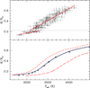 |
Fig. 1. Upper panel: Teff − R diagram for M15 data (including error bars). The solid lines show the fitted linear relationships discussed in the text. Lower panel: Teff − R relationships from theoretical VLM models. Dot-dashed, solid, and dashed lines display 10 Gyr BaSTI-IAC models with [Fe/H] = +0.45, +0.06 and −0.60, respectively. The dotted line shows BASTI-IAC 1 Gyr, [Fe/H] + 0.06 models, while the open circles display the Baraffe et al. (2015) results for 10 Gyr and [Fe/H] = 0.0. |
The lower panel of Fig. 1 displays the theoretical Teff − R relationships for an age of 10 Gyr, [Fe/H] = −0.60, +0.06, and +0.45, and masses between 0.1 and ∼0.6–0.7 M⊙, as derived from the BaSTI-IAC models. In the same diagram we also show the Teff − R relationship for [Fe/H] = 0.06, but an age of 1 Gyr, and the 10 Gyr, [Fe/H] = 0.0 relationship derived from the independent Baraffe et al. (2015) calculations. Theoretical models display a smooth and continuous change in slope of the Teff − R relationship around R ∼ 0.2 R⊙ at temperatures that increase with decreasing [Fe/H]. The assumed stellar age does not affect the shape of the Teff − R relationship, and models from different authors give essentially the same result both qualitatively and quantitatively, at least at metallicities around solar.
For a detailed comparison with the M15 data, we created a synthetic sample of stars with our 10 Gyr BaSTI-IAC grid of models. We employed the same mass and [Fe/H] distribution as were used in the M15 sample, which we show in Fig. 2.
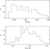 |
Fig. 2. Mass (upper panel) and [Fe/H] (lower panel) number distribution of the M15 M-dwarf sample. |
In brief, for each individual star in the M15 sample, we considered the mass M and [Fe/H] values given by these authors, perturbed by a Gaussian random error with the same 1σ dispersions as given by M15 (typically 0.08 dex for [Fe/H], and about 0.1M for the mass). With these (M, [Fe/H]) pairs we then interpolated amongst the model grid to determine the corresponding theoretical R and Teff values. We repeated this procedure several times to create 100 synthetic counterparts of the M15 sample. In each case, a clear change in slope in the Teff − R relation appears. Figure 3 shows one of our synthetic samples that is representative of the overall result.
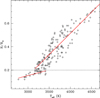 |
Fig. 3. Same as the upper panel of Fig. 2, but for a synthetic sample built using the BASTI-IAC VLM models (see text for details). |
A least-squares linear fit to the data provides R/R⊙ = 0.552(Teff/5777) − 0.133 (with a 1σ dispersion equal to 0.01 around this mean relation) if R/R⊙ < 0.20, and R/R⊙ = 2.094 * (Teff/5777) − 0.936 (with a 1σ dispersion equal to 0.06 around this mean relation) if R/R⊙ > 0.20. These two linear relationships are also shown in Fig. 3. The discontinuity claimed by R19 is retrieved in this synthetic sample, despite the lack of discontinuities in the theoretical models, and it is due to fitting the data in this diagram with linear segments. It reflects the smooth change in slope of the model Teff − R relation.
The synthetic samples qualitatively share the same properties as the observed sample, although there are some differences quantitatively. The change in slope in the Teff − R relation appears at slightly lower radii than in M15. Moreover, the actual values of slopes and zero-points are slightly different from the empirical result. The reason for these differences becomes clear when we examine Fig. 4, which displays fractional differences of R and Teff between the synthetic sample of Fig. 3 and M15, calculated as (observations theory) a function of the M15 Teff estimate.
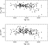 |
Fig. 4. Upper panel: fractional difference (observations-theory) of Teff as a function of the empirical temperatures ( |

For observed Teff values up to ∼3600 K (corresponding to stellar masses ∼0.45 M⊙), there are systematic average constant offsets between theory and observations, and no trends with the empirical Teff. In this range, the average difference in radius is 8±9 % (observed radii are larger) and 3 ± 3 % in Teff (model temperatures are higher). At higher temperatures there are trends with the observed Teff in the direction of both model temperatures and radii becoming increasingly higher and larger compared to observations, and an increasing spread of the differences at a given Teff.
When we varied the age assumed for the stars in the M15 sample from 10 Gyr to 1 Gyr, the results for the slopes in the Teff − R diagram and the differences of R and Teff between models and observations did not change significantly because stars in this mass range evolve very slowly. The change in the model R and Teff for masses up to ∼0.4 M⊙ is almost zero.
2.2. Change in slope of the Teff–R relationship
Figure 5 displays the theoretical M − R and M − Teff diagrams in the VLM regime for an age of 10 Gyr (again, the choice of the age is not critical) and a representative metallicity [Fe/H] = 0.06. The empirical data are also shown. Around 0.2 M⊙, both theoretical and empirical M − Teff relationships display a clear slope change: the effective temperature begins to decrease faster with mass than at higher masses. Figure 5 gives a clearer visual impression of this effect by also showing a comparison between the results of a linear fit to the theoretical relationship in the mass range between 0.4 and 0.25 M⊙, and the actual calculations.
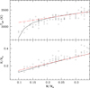 |
Fig. 5. Upper panel: M − Teff relation around M = 0.2 M⊙ for the M15 sample (open circles) and the 10 Gyr BaSTI-IAC models with [Fe/H] = 0.06. Lower panel: same as the upper panel, but for the M − R relation. Dashed red lines in both panels denote linear fits to the model results in the mass range between 0.35 and 0.25 M⊙ (see text for details). |
The same holds true for the radius, even though the effect is not obvious in the data. Analogous to the case of the M − Teff relationship, we display in Fig. 5 a comparison between the linear fit to the theoretical M − R relation in the mass range between 0.4 and 0.25 M⊙, and the actual results. Clearly, the theoretical values for the radius also start to decrease faster with mass when M decreases below ∼0.2 M⊙. This same behaviour of radius and effective temperature with mass is predicted by the Baraffe et al. (2015) models (see also e.g. Burrows et al. 1989; Baraffe & Chabrier 1996; Chabrier & Baraffe 2000). The combination of these two slope changes causes the change in slope of the Teff − R relationship.
The physical origin of this phenomenon is certainly not the transition to fully convective stars, which occurs at higher masses. The culprit is the electron degeneracy, as shown by Chabrier & Baraffe (2000) and with more details by Chabrier & Baraffe (1997); see for example Figs. 6, 12, and 13 in Chabrier & Baraffe (1997). For masses below ∼0.2 M⊙, the electron degeneracy starts to provide a sizable contribution to the gas EOS. Therefore, at around 0.2 M⊙, the model M − R relation begins to change slope (faster decrease with M) to eventually approach the M ∝ R−3 relation below the H-burning limit. As an example, when it is extrapolated at 0.1 M⊙, the M-R linear relation in the regime between 0.4 and 0.25 M⊙ (see Fig. 5) provides a radius equal to ∼0.15 R⊙. The actual calculations give R ∼ 0.125 R⊙, whilst the zero-temperature degenerate M − R relation for solar chemical composition provides R ∼ 0.07 R⊙.
Figure 6 displays the relationships between central temperature (Tc) and M, and the central degeneracy parameter (ψ = kBT/EF, where kB is the Boltzmann constant and EF is the electron Fermi energy) and M, in the same mass range as in Fig. 5. The steady decrease of ψ and Tc with decreasing mass is very clear. The rate of decrease of Tc also changes around 0.2 M⊙. Around this mass, the ever-increasing contribution of the electron degeneracy pressure accelerates the decrease of Tc with M, which in turn causes a faster reduction of the efficiency of the H-burning through the p − p chain. As a consequence, the surface luminosity also decreases faster with decreasing mass below 0.2 M⊙. The trend of the luminosity with M is also shown in Fig. 6, together with the empirical data by M15, which follow the trend predicted by the models.
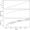 |
Fig. 6. Upper panel: theoretical relationship between central degeneracy parameter and total stellar mass around M = 0.2 M⊙ for 10 Gyr BaSTI-IAC models with [Fe/H] = 0.06. Middle panel: same as the upper panel, but for the central temperature. Lower panel: same as the upper panel, but for the surface luminosity. Data from M15 are also displayed (see text for details). |
The change in slope of the M − Teff relationship in Fig. 5 is then a consequence of the change in the trends of L and R with mass at M = 0.2 M⊙, given that Teff = (L/(4πσR2))1/4 (where σ is the Stefan-Boltzmann constant, see also Chabrier & Baraffe 1997).
3. Summary and conclusions
Recent empirical determinations of mass, effective temperature, and radius for a large sample of M dwarfs (M15, R19) have disclosed an apparent discontinuity in the Teff − R diagram that corresponds to a mass ∼0.2 M⊙. R19 have hypothesised that the reason for this discontinuity is the transition to fully convective stars, although they did not perform any comparison with theory.
Here we have compared a set of existing theoretical VLM models to these observations, to assess whether this discontinuity is predicted by theory, and to determine its physical origin. Theoretical models do not show any discontinuity in the Teff − R diagram, but a smooth change in slope around ∼0.2 M⊙. The discontinuity found by R19 arises from fitting the empirical data with linear segments. To this purpose, we have created synthetic samples of stars with the same [Fe/H], mass, and error distributions as the observations, fitting the resulting Teff − R diagram with linear segments, as done by R19. Despite some small offsets between the Teff and R scale of the models and the observations, the linear fits show a discontinuity that corresponds to a mass ∼0.2 M⊙, where the theoretical models display a smooth change in slope. As discussed by Chabrier & Baraffe (1997), this smooth change in slope of the models reflects the growing contribution of the electron degeneracy to the gas EOS below ∼0.2 M⊙, and not the transition to fully convective stars, which is predicted to occur at ∼0.35 M⊙. A stronger electron degeneracy causes a faster decrease of R with decreasing M, and a faster decrease of both central temperature and luminosity with decreasing M. These in turn induce a steeper decrease of Teff with M. These changes in slope of the M − R and M − Teff produce a corresponding change in the Teff − R diagram. The empirical results by M15 and R19 therefore provide a clear signature of the threshold beyond which the electron degeneracy provides an important contribution to the stellar EOS. These data are therefore an additional test of the consistency of the theoretical framework for VLM models.
Models are publicly available at the following URL: http://basti-iac.oa-abruzzo.inaf.it
Acknowledgments
SC acknowledges support from Premiale INAF MITiC, from INFN (Iniziativa specifica TAsP), PLATO ASI-INAF contract n.2015-019-R0 and n.2015-019-R.1-2018, and grant AYA2013-42781P from the Ministry of Economy and Competitiveness of Spain. The authors acknowledge the anonymous referee for pointing out the discussion in Sect. 3.1.1. of Chabrier & Baraffe (1997).
References
- Allard, F., Homeier, D., & Freytag, B. 2012, Phil. Trans. R. Soc. London Ser. A, 370, 2765 [Google Scholar]
- Anglada-Escudé, G., Amado, P. J., Barnes, J., et al. 2016, Nature, 536, 437 [NASA ADS] [CrossRef] [PubMed] [Google Scholar]
- Baraffe, I., & Chabrier, G. 1996, ApJ, 461, L51 [NASA ADS] [CrossRef] [Google Scholar]
- Baraffe, I., Homeier, D., Allard, F., & Chabrier, G. 2015, A&A, 577, A42 [NASA ADS] [CrossRef] [EDP Sciences] [Google Scholar]
- Böhm-Vitense, E. 1958, Z. Astrophys., 46, 108 [Google Scholar]
- Burrows, A., Hubbard, W. B., & Lunine, J. I. 1989, ApJ, 345, 939 [NASA ADS] [CrossRef] [Google Scholar]
- Caffau, E., Ludwig, H.-G., Steffen, M., Freytag, B., & Bonifacio, P. 2011, Sol. Phys., 268, 255 [NASA ADS] [CrossRef] [Google Scholar]
- Cassisi, S., Salaris, M., & Irwin, A. W. 2003, ApJ, 588, 862 [NASA ADS] [CrossRef] [Google Scholar]
- Cassisi, S., Potekhin, A. Y., Pietrinferni, A., Catelan, M., & Salaris, M. 2007, ApJ, 661, 1094 [NASA ADS] [CrossRef] [Google Scholar]
- Chabrier, G., & Baraffe, I. 1997, A&A, 327, 1039 [NASA ADS] [Google Scholar]
- Chabrier, G., & Baraffe, I. 2000, ARA&A, 38, 337 [NASA ADS] [CrossRef] [Google Scholar]
- Cox, J. P., & Giuli, R. T. 1968, Principles of Stellar Structure (New York: Gordon and Breach) [Google Scholar]
- Feiden, G. A., & Chaboyer, B. 2012, ApJ, 757, 42 [NASA ADS] [CrossRef] [Google Scholar]
- Ferguson, J. W., Alexander, D. R., Allard, F., et al. 2005, ApJ, 623, 585 [NASA ADS] [CrossRef] [Google Scholar]
- Hidalgo, S. L., Pietrinferni, A., Cassisi, S., et al. 2018, ApJ, 856, 125 [NASA ADS] [CrossRef] [Google Scholar]
- Iglesias, C. A., & Rogers, F. J. 1996, ApJ, 464, 943 [NASA ADS] [CrossRef] [Google Scholar]
- Mann, A. W., Feiden, G. A., Gaidos, E., Boyajian, T., & von Braun, K. 2015, ApJ, 804, 64 [NASA ADS] [CrossRef] [Google Scholar]
- Parsons, S. G., Gänsicke, B. T., Marsh, T. R., et al. 2018, MNRAS, 481, 1083 [NASA ADS] [CrossRef] [Google Scholar]
- Quintana, E. V., Barclay, T., Raymond, S. N., et al. 2014, Science, 344, 277 [NASA ADS] [CrossRef] [PubMed] [Google Scholar]
- Rabus, M., Lachaume, R., Jordán, A., et al. 2019, MNRAS, 484, 2674 [NASA ADS] [CrossRef] [Google Scholar]
- Rauer, H., Catala, C., Aerts, C., et al. 2014, Exp. Astron., 38, 249 [NASA ADS] [CrossRef] [Google Scholar]
- Ricker, G. R., Winn, J. N., Vanderspek, R., et al. 2015, J. Astron. Telesc. Instrum. Syst., 1, 014003 [NASA ADS] [CrossRef] [Google Scholar]
- Rogers, F. J., & Nayfonov, A. 2002, ApJ, 576, 1064 [Google Scholar]
- Saumon, D., Chabrier, G., & van Horn, H. M. 1995, ApJS, 99, 713 [NASA ADS] [CrossRef] [Google Scholar]
- Shields, A. L., Ballard, S., & Johnson, J. A. 2016, Phys. Rep., 663, 1 [NASA ADS] [CrossRef] [Google Scholar]
- Spada, F., Demarque, P., Kim, Y.-C., & Sills, A. 2013, ApJ, 776, 87 [NASA ADS] [CrossRef] [Google Scholar]
- Tognelli, E., Prada Moroni, P. G., & Degl’Innocenti, S. 2018, MNRAS, 476, 27 [Google Scholar]
- Torres, G., Andersen, J., & Giménez, A. 2010, A&ARv, 18, 67 [Google Scholar]
All Figures
|
Fig. 1. Upper panel: Teff − R diagram for M15 data (including error bars). The solid lines show the fitted linear relationships discussed in the text. Lower panel: Teff − R relationships from theoretical VLM models. Dot-dashed, solid, and dashed lines display 10 Gyr BaSTI-IAC models with [Fe/H] = +0.45, +0.06 and −0.60, respectively. The dotted line shows BASTI-IAC 1 Gyr, [Fe/H] + 0.06 models, while the open circles display the Baraffe et al. (2015) results for 10 Gyr and [Fe/H] = 0.0. |
| In the text | |
|
Fig. 2. Mass (upper panel) and [Fe/H] (lower panel) number distribution of the M15 M-dwarf sample. |
| In the text | |
|
Fig. 3. Same as the upper panel of Fig. 2, but for a synthetic sample built using the BASTI-IAC VLM models (see text for details). |
| In the text | |
|
Fig. 4. Upper panel: fractional difference (observations-theory) of Teff as a function of the empirical temperatures ( |
| In the text | |
|
Fig. 5. Upper panel: M − Teff relation around M = 0.2 M⊙ for the M15 sample (open circles) and the 10 Gyr BaSTI-IAC models with [Fe/H] = 0.06. Lower panel: same as the upper panel, but for the M − R relation. Dashed red lines in both panels denote linear fits to the model results in the mass range between 0.35 and 0.25 M⊙ (see text for details). |
| In the text | |
|
Fig. 6. Upper panel: theoretical relationship between central degeneracy parameter and total stellar mass around M = 0.2 M⊙ for 10 Gyr BaSTI-IAC models with [Fe/H] = 0.06. Middle panel: same as the upper panel, but for the central temperature. Lower panel: same as the upper panel, but for the surface luminosity. Data from M15 are also displayed (see text for details). |
| In the text | |
Current usage metrics show cumulative count of Article Views (full-text article views including HTML views, PDF and ePub downloads, according to the available data) and Abstracts Views on Vision4Press platform.
Data correspond to usage on the plateform after 2015. The current usage metrics is available 48-96 hours after online publication and is updated daily on week days.
Initial download of the metrics may take a while.