| Issue |
A&A
Volume 592, August 2016
The XXL Survey: First results
|
|
|---|---|---|
| Article Number | A10 | |
| Number of page(s) | 7 | |
| Section | Catalogs and data | |
| DOI | https://doi.org/10.1051/0004-6361/201526818 | |
| Published online | 15 June 2016 | |
The XXL Survey
XI. ATCA 2.1 GHz continuum observations⋆
1 University of Zagreb, Physics Department, Bijenička cesta 32, 10002 Zagreb, Croatia
e-mail: vs@phy.hr
2 International Centre for Radio Astronomy Research (ICRAR), M468, University of Western Australia, 35 Stirling Hwy, WA 6009, Australia
3 Istituto di Radioastronomia di Bologna – INAF, via P. Gobetti, 101, 40129 Bologna, Italy
4 INAF–Osservatorio Astronomico di Bologna, via Ranzani 1, 40127 Bologna, Italy
5 H.H. Wills Physics Laboratory, University of Bristol, Tyndall Avenue, Bristol BS8 1TL, UK
6 INAF, IASF Milano, via Bassini 15, 20133 Milano, Italy
7 Laboratoire Lagrange, Université Côte d’Azur, Observatoire de la Côte d’Azur, CNRS, Blvd de l’Observatoire, CS 34229, 06304 Nice Cedex 4, France
8 Department of Astronomy, University of Geneva, Ch. d’Ecogia 16, 1290 Versoix, Switzerland
9 Dept. of Earth & Space Sciences, Chalmers University of Technology, Onsala Space Observatory, 439 92 Onsala, Sweden
10 School of Physics and Astronomy, University of Birmingham, Edgbaston, Birmingham B15 2TT, UK
11 Argelander Institut für Astronomie, Universität Bonn, 53121 Bonn, Germany
12 Service d’Astrophysique AIM, CEA/DSM/IRFU/SAp, CEA Saclay, 91191 Gif-sur-Yvette, France
13 Leiden Observatory, Leiden University, PO Box 9513, 2300 RA Leiden, The Netherlands
14 Dipartimento di Fisica e Astronomia Universita degli Studi di Bologna, Viale Berti Pichat 6/2, 40127 Bologna, Italy
Received: 23 June 2015
Accepted: 13 October 2015
We present 2.1 GHz imaging with the Australia Telescope Compact Array (ATCA) of a 6.5 deg2 region within the XXM-Newton XXL South field using a band of 1.1−3.1 GHz. We achieve an angular resolution of 4.7′′ × 4.2′′ in the final radio continuum map with a median rms noise level of 50 μJy/beam. We identify 1389 radio sources in the field with peak S/N ≥ 5 and present the catalogue of observed parameters. We find that 305 sources are resolved, of which 77 consist of multiple radio components. These number counts are in agreement with those found for the COSMOS-VLA 1.4 GHz survey. We derive spectral indices by a comparison with the Sydney University Molongolo Sky Survey (SUMSS) 843 MHz data. We find an average spectral index of − 0.78 and a scatter of 0.28, in line with expectations. This pilot survey was conducted in preparation for a larger ATCA program to observe the full 25 deg2 southern XXL field. When complete, the survey will provide a unique resource of sensitive, wide-field radio continuum imaging with complementary X-ray data in the field. This will facilitate studies of the physical mechanisms of radio-loud and radio-quiet AGNs and galaxy clusters, and the role they play in galaxy evolution. The source catalogue is publicly available online via the XXL Master Catalogue browser and the Centre de Données astronomiques de Strasbourg (CDS).
Key words: radio continuum: galaxies / X-rays: galaxies / surveys / galaxies: evolution / galaxies: clusters: general
The ATCA Catalogue is available at the CDS via anonymous ftp to cdsarc.u-strasbg.fr (130.79.128.5) or via http://cdsarc.u-strasbg.fr/viz-bin/qcat?J/A+A/592/A10
© ESO, 2016
1. Introduction
Low-luminosity radio-loud AGN (L1.4 GHz ≲ 1025 W/Hz) are somewhat puzzling systems which do not fit into the Unified Model of AGN (e.g. Antonucci 1993). They are predominantly found in quiescent galaxies and are often at the centres of groups or clusters, are likely fuelled by radiatively inefficient accretion of hot gas, and would not be identified as AGNs at any other wavelength (e.g. Hardcastle et al. 2007; Smolčić et al. 2008, 2009a,b; Hickox et al. 2009). These AGNs are believed to significantly affect the evolution of their host galaxies and perhaps of their environment on larger scales (e.g. Croton et al. 2006; Fabian et al. 2006). For example, mechanical energy transfer via the radio jets may heat the intra-cluster/group gas and the gaseous halo of the host galaxy, both of which are best traced via X-rays (e.g. Fabian et al. 2006). This heating – deemed crucial in cosmological models of galaxy formation – is referred to as feedback; however, it is still not completely understood on group/cluster scales or on galaxy scales. In simulations of galaxy formation and evolution, such radio-mode feedback plays a critical role in suppressing massive galaxy formation and reproducing various observed galaxy properties (e.g. Croton et al. 2006). While this has been studied for individual cases (e.g. Worrall et al. 2012), robust observational information relating to these feedback processes is limited by the lack of statistically large samples of radio sources (Best et al. 2006; Merloni & Heinz 2008; Smolčić et al. 2009a).
To comprehensively examine the role of AGN feedback on their hosts and environments, it is essential to obtain both radio and X-ray coverage over large fields. This synergy allows a direct insight into different heating mechanisms (thermal versus non-thermal) as a function of redshift, source type, and galaxy location in large-scale structures. An example of a previous radio survey with available X-ray coverage is the VLA-COSMOS survey (Schinnerer et al. 2007; Smolčić et al. 2014) with X-ray data from the XMM-Newton and Chandra observatories (Hasinger et al. 2007; Elvis et al. 2009; Civano et al. 2012, 2015). This is a deep radio survey, reaching a sensitivity of ~15 μJy/beam at 20 cm, but only covering a 2 deg2 field. Another example is the Boötes survey (Hickox et al. 2009; de Vries et al. 2002), which covers a wider field (7 deg2) but is shallower (rms ~28 μJy/beam at 20 cm). To accurately measure the evolution of the radio galaxy luminosity function, particularly at the bright end, it is necessary to conduct very wide-field radio/X-ray surveys while maintaining good sensitivity. For this purpose, we present the first results from the pilot program of a large radio continuum survey with the Australia Telescope Compact Array (ATCA) to cover 25 deg2 of the XXL survey field.
The XXL survey comprises the largest XMM-Newton project approved to date (Pierre et al. 2016, Paper I hereafter); it has provided 3 Ms of new data, and more than 6 Ms when including archival data. The main goals of this X-ray survey are to provide long-lasting legacy data for studies of galaxy clusters and AGNs and to constrain the dark energy equation of state using clusters of galaxies. Observations with XMM-Newton are essentially complete; a few fields are undergoing re-observation. The survey covers an equatorial and a southern region of ~25 deg2 each, down to a point-source sensitivity of ~5 × 10-15 erg s-1 cm-2 (0.5−2 keV). Several thousand spectroscopic redshifts of X-ray luminous sources have been collected with the Anglo-Australian Telescope (Lidman et al. 2016, Paper XIV) and photometric redshifts from existing optical/near-IR (NIR) data will reach accuracies better than ~10% (Fotopoulou et al. 2016, Paper VI). See Paper I for an overview of the survey.
To provide the complementary radio data, we are undertaking a large survey with ATCA to cover the full southern XXL field (hereafter XXL-S) at 2.1 GHz to an expected sensitivity of ~43 μJy. These observations will provide a unique resource of sensitive, complementary radio and X-ray coverage over the widest field to date. This will allow detailed studies of the role of radio-mode feedback on the formation and evolution of massive galaxies and galaxy clusters.
Here we report the results of the pilot survey covering the central 6.5 deg2 of the field. We achieve a spatial resolution of ~4′′ and an average rms of ~50 μJy/beam. We have identified 1389 radio sources in the field. Section 2 of this paper details the ATCA observations, Sect. 3 discusses the data reduction and imaging strategy, Sect. 4 presents the source identification and catalogue, and Sect. 5 provides the summary.
2. Observations, data reduction, and imaging
2.1. Observations
We conducted 2.1 GHz observations with ATCA1 over 37 h on 3−6 September 2012 in the 6A (6 km) configuration and over 15 h on 25−26 November 2012 in the 1.5C (1.5 km) configuration. The observations were performed using the Compact Array Broadband Backend (CABB; Wilson et al. 2011) correlator, which covers a full 2 GHz bandwidth centred on 2.1 GHz using a channel width of 1 MHz. To cover the 6.5 deg2 pilot field, 81 mosaic pointings were placed in a layout such that the separation between adjacent pointings in right ascension (RA) and declination (Dec) was two-thirds of the primary beam full-width at half-maximum (FWHM) at 2.1 GHz, i.e. 14.7 arcmin. We used source 1934-638 as the primary calibrator, and observed it during each observing run for 10 min on-source. The flux density of 1934-638 was tied to the widely used absolute flux density scale of Baars et al. (1977), as described in Reynolds (1994). Source 2333-528 was taken as the secondary calibrator and it was observed for 2 min on-source every 32 min between observations of different sets of pointings.
2.2. Data reduction
We used the Multichannel Image Reconstruction, Image Analysis and Display (miriad) software package to reduce the data. In the calibration step we used 16 frequency bins in the GPCAL (gain/phase/polarisation calibration) task (i.e. bin width of 128 MHz). The 81 pointings were individually reduced and imaged. Automated flagging was performed using the MIRIAD task PGFLAG. This is based on AOFLAGGER and was developed for LOFAR data sets, but has now been applied to various radio data from other instruments (Offringa et al. 2010, 2012). We found that the lowest frequency sub-band, which was centred at 1.204 GHz, was significantly affected by radio frequency interference (RFI). In the shortest baselines 80–90 percent of the data in this sub-band was flagged, and even in the long 6 km baselines 60–70 percent of the data was affected by RFI. Consequently, this sub-band was discarded completely.
2.3. Imaging
Wideband receivers such as CABB on the ATCA present new challenges to radio imaging. The primary beam response, the synthesised beam, and the flux density of most sources vary significantly with frequency over the 2 GHz wide bandwidth. One method used to mitigate these issues is to divide (u,v) data into sub-bands and then to force similar beam sizes with an appropriate “robustness” parameter (Briggs 1995). This approach was used to image VLA data spanning 2–4 GHz (Condon et al. 2012; Novak et al. 2015; Smolčić et al. 2015). We tested two imaging schemes, one where the (u,v) data are not divided into sub-bands and a second scheme where the 2048 MHz CABB band is divided into 256 MHz sub-bands. We find that the effect of bandwidth smearing is more significant in the first approach, thus hereafter we focus and describe in detail only the second imaging approach.
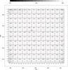 |
Fig. 1 Inverted greyscale of our XXL-S Pilot Survey mosaic at 2.1 GHz. The greyscale colourbar in units of mJy/beam is shown at the top. Overlaid are histograms of pixel flux distributions for different regions of the mosaic. The standard deviation for each region is indicated in each panel (in units of μJy/beam). The x-axis of the histograms shows flux density in μJy/beam and the y-axis shows counts. The outer 500 pixels of the map have been excluded here since they are not considered in the source-finding process. |
The calibrated data set of each pointing was split into eight sub-bands of 256 MHz each. As the lowest sub-band is almost entirely contaminated by RFI it was disregarded. Each sub-band was imaged with a robust weighting chosen to match the beam sizes across the seven remaining sub-bands. Multifrequency cleaning and self-calibration were performed for each pointing and each sub-band. The task MFCLEAN was used to perform cleaning; the clean region was set to the inner 23′ region of the image because a “border” is required for MFCLEAN. The cleaned region extends beyond the 7% primary beam response level at 2.1 GHz, the effective frequency of the observations, therefore encompassing the full region of interest. We performed two iterations of phase self-calibration to improve the images. The first self-calibration iteration was performed with a model generated by cleaning to 10σ (i.e. bright sources only) and a second model generated by cleaning to 6σ. The individual images were restored with the same beam, i.e. the average beam of the 7 × 81 images, 4.7″ × 4.2″. The final sub-band combined mosaic was then obtained by using the LINMOS task to create a noise-weighted mosaic of all 7 × 81 images. The different primary beam sizes for different sub-bands will result in different effective frequencies for different positions in the mosaic (see Condon et al. 2012 for details). To take this into account we generated a mosaic of effective frequencies using the task LINMOS. The effective frequency of the central 5.2 deg2 region of the image has a median of 2.10 GHz and a standard deviation of only 0.07 GHz.
The final mosaic, with an angular resolution of 4.7″ × 4.2″ and a pixel size of ~1′′ × 1′′, is shown in Fig. 1. We also overlaid the pixel flux distribution in 12 × 12 regions over the mosaic. The main image artefacts are stripes from imperfect cleaning of sidelobes around bright sources and what are known as chequerboard artefacts around bright extended sources caused by missing short baselines. The cleaning artefacts are caused by a variety of factors, including imperfect antenna calibration and imperfect models for cleaning. For example, MFCLEAN can only model the spectral energy distribution of a source as a power law in log space (S ∝ να) and it uses only point sources in the deconvolution. To improve on this, the new ATCA observations of the full 25 deg2 field have been performed with a more complete uv-coverage, and we are developing a rigorous cleaning process to reduce sidelobes around the bright sources and peeling (e.g. Intema et al. 2009) of off-axis bright sources to reduce the artefacts in neighbouring pointings. This will allow us to minimise the rms of the image and to identify and catalogue sources down to a 5σ level with a high level of completeness. In Fig. 2 we show the mosaic sensitivity function, i.e. the total area covered at a given rms. The mosaic reaches a median rms of 50 μJy/beam.
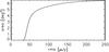 |
Fig. 2 Mosaic sensitivity function showing the total area with a noise level below a given rms. |
3. Source catalogue
3.1. Noise image
In order to select a sample of radio sources above a given threshold, defined in terms of local signal-to-noise ratio (S/N), we derived a noise image using the task RMSD in the Astronomical Image Processing System (AIPS). The rms was calculated for each pixel based on the data in the box surrounding the pixel. The size of the box was chosen to be 60 pixels (i.e. 60′′ × 60′′). The rms was calculated on a multi-iteration basis, which excludes the points that are more than 3 times the rms derived from the previous iteration until convergence is reached. The noise distribution is not entirely Gaussian owing to the presence of residual sidelobes around the many bright radio sources in the field. The median rms is 50 μJy/beam. About 3% of the noise values are higher than 200 μJy and are located around the brightest sources in the mosaic. Using the total intensity and noise images we produced a S/N map. The minimum and maximum values of this S/N map are − 7.5 and 1006, respectively.
3.2. Source detections
To extract a catalogue of sources we followed the procedure already applied to the COSMOS field and tested by Schinnerer et al. (2007, 2010) and Smolčić et al. (2014). We first ran the aips task SAD on the S/N map to derive a catalogue of radio components. At this stage, we used a threshold of 4.7 in peak S/N. For each selected component, the peak surface brightness (hereafter peak flux), the total flux density, the position, and the size were estimated using a Gaussian fit. However, for faint components the optimal estimate of the peak flux and of the component position were obtained by a non-parametric interpolation of the pixel values around the fitted position using the task MAXFIT in aips (as in Schinnerer et al. 2007). Only the components with a S/N (derived as the ratio between the MAXFIT peak brightness and the local noise at the position of the MAXFIT peak) ≥5 are included in the catalogue. Around the brightest sources (~50 mJy/beam) residual sidelobes can be mistakenly identified as real components by SAD. These regions were inspected by eye to remove sidelobe spikes. We further excluded all data less than 500 pixels (i.e. 500′′) from the outer edge of the noise map where the rms is too large for reliable source-finding.
Some of the components identified by SAD clearly belong to a single radio source, for example the two lobes of FRII radio sources (Fanaroff & Riley 1974) or extended emission associated with compact components. We visually checked all these cases and compared them with available deep optical images (from the Blanco Cosmology Telescope (BCS) and also DECcam and VISTA-NIR images; see Paper I and references therein) in order to associate multiple components with a single radio source. If an optical counterpart can be found, this often helps to determine whether two radio components are associated with one central galaxy. An example of such a multicomponent system is shown in Fig. 3.
Other automatic methods that are based on a statistical approach could also be used to identify multiple radio components belonging to a single source; however, our experience has taught us that a classification based on the radio morphology of the component supported by deep optical/NIR images is more effective. This task is clearly time consuming for large surveys, but it will be adopted for the whole survey.
The final catalogue lists 1389 radio sources with S/N ≥ 5. Of these, 77 are multiple, i.e. fitted with at least two separate components. For the multicomponent sources we recalculated the flux using the aips task TVSTAT which allows the manual definition of the integration bounds, which we set to 2σ contours. In the catalogue this value is reported for the total flux, the peak flux is set to − 99, and the sources are flagged as multicomponent sources (MULT = 1).
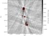 |
Fig. 3 Example of a multicomponent source. The greyscale 2.1 GHz image is shown in the background; the red radio flux contours are shown at 0.8, 1.6, 3.2, 6.4, 12.8 mJy/beam. |
Figure 4 shows the ratio of total flux (ST) to peak flux (SP) versus the S/N of the catalogued single-component sources. As described in Bondi et al. (2003), this plot can be used to distinguish between point (unresolved) sources and extended (resolved) sources. In this figure, the vertical offset from 1.0 at the very bright end is caused by bandwidth smearing in the mosaic (see insert in Fig. 4 and Bondi et al. 2008 for details). Bandwidth smearing affects the fluxes in such a way that the peak flux decreases by a certain amount, while the total flux remains the same. Based on the data shown in Fig. 4, we estimated a 4% bandwidth smearing effect, and thus corrected all peak fluxes by multiplying them by 1.04. Accordingly, following Bondi et al. (2003, 2008) we fitted a lower envelope to the data, which contains 90% of the sources with ST<SP (with SP corrected for the 4% bandwidth smearing), and mirrored it above ST/SP = 1.00. The upper envelope, above which sources are considered resolved, is then given by 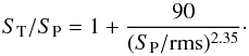 (1)In total we find 228 single-component sources to be resolved (in addition to the 77 multicomponent sources). The resolved sources are flagged in the catalogue by RES = 1. For the unresolved sources, the total flux density is set equal to the peak flux density and the angular size is set equal to zero in the catalogue.
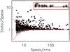 |
Fig. 4 Ratio of total to peak flux of sources identified in the 2 GHz mosaic versus the peak flux to rms ratio. Also shown are the boundary encompassing 90% of the sources (lower line) and its reflection about the ratio = 1 value (upper line), above which the sources are considered to be resolved (marked by open symbols). The inset shows a magnified view of the high Speak region (roughly 180 <Speak/ rms < 450) where the vertical offset from 1.0 due to the bandwidth smearing is clearly visible (see Sect. 3.2). |
Finally, we calculated the uncertainties σST and σSP on the total (ST) and peak (SP) fluxes using the method described in detail in Condon (1997, see also Schinnerer et al. 2007),  /ρ2 and
  /ρ2, where ρ is the signal to noise ratio given by
 ![\begin{eqnarray*} \rho^{2}=\frac{\theta_{\rm M}\theta_{\rm m}}{4\theta_{\rm N}^{2}}\left[1+\left(\frac{\theta_{\rm N}}{\theta_{\rm M}}\right)^{2}\right]^{3/2}\left[1+\left(\frac{\theta_{\rm N}}{\theta_{\rm m}}\right)^{2}\right]^{3/2}\frac{S_{\rm P}^{2}}{\sigma_{\rm map}^{2}} \end{eqnarray*}](/articles/aa/full_html/2016/08/aa26818-15/aa26818-15-eq48.png) where θM and θm are the fitted FWHMs of the major and minor axes, σmap is the noise of the image, and θN is the FWHM of the synthesised beam.
where θM and θm are the fitted FWHMs of the major and minor axes, σmap is the noise of the image, and θN is the FWHM of the synthesised beam.
The positional errors are estimated using 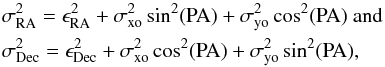 where PA is the positional angle of the major axis,
  and
and  are the calibration errors, while σxo and σyo are
  (4 ln 2)ρ2 and
  /(4 ln 2)ρ2, respectively. Calibration terms and must be estimated from comparison with external data with better positional accuracy than the one tested. We calculated our calibration terms from the comparison between the position of single-component XXL ATCA radio sources with S/N> 10 and their optical counterpart (62 sources in total). The mean values and standard deviations found from this comparison are ΔRA = 0.24 ± 0.34 arcsec and ΔDec = −0.12 ± 0.22 arcsec. These position offsets are barely significant (6 and 4 times the error on the mean, respectively). Given the size of the beam and the error associated with the position of the bulk of weaker sources (comparable to or larger than the previous offsets) at this stage we assume no significant offset between the radio and optical frames. Once the full XXL-S field has been covered, we plan to investigate in greater detail any possible systematic and/or position-dependent offsets between the radio and optical positions. Therefore, in the error budget we assume a calibration error
  arcsec in RA and
  arcsec in Dec.
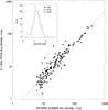 |
Fig. 5 Comparison between SUMSS 843 MHz and ATCA-XXL 2.1 GHz fluxes for the XXL-S Pilot area based on 159 sources detected in the shallower (rms ~1.25 mJy/beam) SUMSS survey. The inset shows the spectral index distribution for the sources with a mean of − 0.78 and a standard deviation of 0.28. The solid line corresponds to a spectral index of − 0.78. |
An example page of the final source catalogue is shown in Table 1. The full catalogue is available as a queryable database table “XXL_ATCA_15” via the XXL Master Catalogue browser2. A copy is also available at the Centre de Données astronomiques de Strasbourg (CDS).
Sample catalogue page.
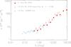 |
Fig. 6 Normalised differential source counts for the 2.1 GHz ATCA XXL-S survey (red filled dots), estimated 1.4 GHz ATCA XXL-S counts (assuming a spectral index of − 0.78; red open dots) and for the COSMOS VLA 1.4 GHz survey (blue open squares). |
4. Comparison with other radio data
4.1. Flux comparison and spectral indices
In the radio regime, the area of XXL-S is covered (with sufficient sensitivity for comparison) by the Sydney University Molonglo Sky Survey (SUMSS) survey3 (Bock et al. 1999; Mauch et al. 2003). Completed in 2007, SUMSS was conducted at 843 MHz and an angular resolution of 45″ × 45″cosec | δ |, and it covers almost the whole sky south of Declination − 30 deg. The SUMSS source catalogue (Mauch et al. 2003) lists sources brighter than 6 mJy/beam in peak flux. Cross-correlating our 2.1 GHz source catalogue with the SUMSS survey catalogue using a radius of 15″, we find 159 matches after excluding faint multiple sources blended in the SUMSS data. A comparison of the 2.1 GHz ATCA and 843 MHz SUMSS fluxes for these sources is shown in Fig. 5. Also shown is the spectral index distribution of the sources; the spectral index (α) is defined such that Sν ∝ να, where Sν is the flux at frequency ν. A Gaussian fit to the spectral index distribution yields a mean of − 0.78 and a standard deviation of 0.28. These values are consistent with expectations (e.g. Kimball & Ivezić 2008).
4.2. XXL ATCA source counts
In this section we report the 2.1 GHz radio source counts obtained in our ATCA observation in the XXL-S field. The completeness of the sample will be tested with the appropriate simulation (see Bondi et al. 2003 for the description of the method) when the full radio data set becomes available over the entire XXL-S field. Therefore, in order to reduce problems with possible spurious sources near the flux limit and the effects of incompleteness, we construct the 2.1 GHz ATCA radio source counts considering only the 1003 sources in the pilot survey with a flux density greater than 0.35 mJy, corresponding to S/N ≳ 7.0 (assuming an average rms of 0.05 mJy, see Sect. 3.1).
The source counts from our pilot sample are summarised in Table 2 where, for each flux density bin, we report the minimum and mean flux density, the observed number of sources, the differential source density n = dN/ dS (in sr-1 Jy-1), the normalised differential counts nS2.5 (in sr-1 Jy1.5) with the estimated Poisson error (as n1 / 2S2.5), and the integrated counts N( >S) (in deg-2).
The 2.1 GHz radio source counts for the pilot sample in the XXL-S survey.
The normalised differential counts nS2.5 are plotted in Fig. 6 where, for comparison, the differential source counts obtained from the COSMOS VLA survey at 1.4 GHz (Bondi et al. 2008) are also plotted. For ease of comparison, the estimated ATCA source counts at 1.4 GHz are also plotted assuming a spectral index of − 0.78 for all sources (i.e. the average value derived in Sect. 4.1). We extrapolate the 7σ cutoff of 0.35 mJy at 2.1 GHz to 1.4 GHz using the average spectral index of α = −0.78, i.e. the 1.4 GHz extrapolated counts are cut off at 0.48 mJy. As shown in Fig. 6, our counts are in good agreement with the COSMOS survey counts over the full flux density range sampled by our survey (~0.35−100 mJy), indicating that the survey is relatively complete, at least down to 7σ.
5. Summary
We have presented a 2.1 GHz ATCA continuum map of the central 6.5 deg2 of the southern XXL field. This pilot survey is part of a larger observing program currently underway to map the full 25 deg2 XXL-S field. This will provide sensitive, wide-field continuum data with complementary X-ray coverage allowing detailed studies of the heating mechanisms of radio AGN and galaxy clusters.
Our final continuum map has an angular resolution of 4.7″ × 4.2″ and an rms of ~50 μJy/beam. There are 1389 radio sources above 5σ identified in the map, 77 of which consist of multiple components. The differential source counts are consistent with those found in the COSMOS-VLA survey at 1.4 GHz. By comparing the 2.1 GHz ATCA fluxes with the 843 MHz SUMSS survey, we find an average spectral index for these sources of − 0.78 with a scatter of 0.28, which is consistent with previous findings.
The ATCA observations of the remainder of the XXL-S field have been completed and data reduction is underway. The focus is now on developing a rigorous cleaning process to reduce sidelobes around the bright continuum sources, to minimise the rms of the image, and to identify and catalogue sources down to a ~5σ level with good completeness.
Acknowledgments
XXL is an international project based on an XMM Very Large Programme surveying two 25 deg2 extragalactic fields at a depth of ~5 × 10-15 erg cm-2 s-1 in the [0.5−2] keV band for point-like sources. The XXL website is http://irfu.cea.fr/xxl. Multiband information and spectroscopic follow-up of the X-ray sources are obtained through a number of survey programmes, summarised at http://xxlmultiwave.pbworks.com/. The Australia Telescope Compact Array is part of the Australia Telescope National Facility which is funded by the Commonwealth of Australia for operation as a National Facility managed by CSIRO. This research was funded by the European Union’s Seventh Framework program under grant agreement 333654 (CIG, “AGN feedback”). V.S., J.D. and M.N. acknowledge funding from the European Union’s Seventh Framework program under grant agreement 337595 (ERC Starting Grant, “CoSMass”). V.S. acknowledges funding from the Australian Group of Eight European Fellowships 2013. F.P. acknowledges support from the BMBF/DLR grant 50 OR 1117, the DFG grant RE 1462-6 and the DFG Transregio Programme TR33. M.N.B. and M. Birkinshaw acknowledge funding from the UK’s STFC. H.R. acknowledges support from the ERC Advanced Investigator program NewClusters 321271.
References
- Antonucci, R. 1993, ARA&A, 31, 473 [Google Scholar]
- Baars, J. W. M., Genzel, R., Pauliny-Toth, I. I. K., & Witzel, A. 1977, A&A, 61, 99 [NASA ADS] [Google Scholar]
- Best, P. N., Kaiser, C. R., Heckman, T. M., & Kauffmann, G. 2006, MNRAS, 368, L67 [NASA ADS] [Google Scholar]
- Bock, D. C.-J., Large, M. I., & Sadler, E. M. 1999, AJ, 117, 1578 [NASA ADS] [CrossRef] [Google Scholar]
- Bondi, M., Ciliegi, P., Zamorani, G., et al. 2003, A&A, 403, 857 [NASA ADS] [CrossRef] [EDP Sciences] [Google Scholar]
- Bondi, M., Ciliegi, P., Schinnerer, E., et al. 2008, ApJ, 681, 1129 [NASA ADS] [CrossRef] [Google Scholar]
- Briggs, D. S. 1995, BAAS, 27, 112.02 [Google Scholar]
- Civano, F., Elvis, M., Brusa, M., et al. 2012, ApJS, 201, 30 [NASA ADS] [CrossRef] [Google Scholar]
- Civano, F., Marchesi, S., Comastri, A., et al. 2015, ApJ, submitted [Google Scholar]
- Condon, J. J., Cotton, W. D., Fomalont, E. B., et al. 2012, ApJ, 758, 23 [NASA ADS] [CrossRef] [Google Scholar]
- Croton, D. J., Springel, V., White, S. D. M., et al. 2006, MNRAS, 365, 11 [NASA ADS] [CrossRef] [Google Scholar]
- de Vries, W. H., Morganti, R., Röttgering, H. J. A., et al. 2002, AJ, 123, 1784 [NASA ADS] [CrossRef] [Google Scholar]
- Elvis, M., Civano, F., Vignali, C., et al. 2009, ApJS, 184, 158 [NASA ADS] [CrossRef] [Google Scholar]
- Fabian, A. C., Sanders, J. S., Taylor, G. B., et al. 2006, MNRAS, 366, 417 [Google Scholar]
- Fanaroff, B. L., & Riley, J. M. 1974, MNRAS, 167, 31 [NASA ADS] [CrossRef] [Google Scholar]
- Fotopoulou, S., Pacaud, F., Paltani, S., et al. 2016, A&A, 592, A5 (XXL Survey, VI) [NASA ADS] [CrossRef] [EDP Sciences] [Google Scholar]
- Hardcastle, M., Evans, D., & Croston, J. 2007, MNRAS, 376, 1849 [NASA ADS] [CrossRef] [Google Scholar]
- Hasinger, G., Cappelluti, N., Brunner, H., et al. 2007, ApJS, 172, 29 [NASA ADS] [CrossRef] [Google Scholar]
- Hickox, R. C., Jones, C., Forman, W. R., et al. 2009, ApJ, 696, 891 [Google Scholar]
- Kimball, A. E., & Ivezić, Ž. 2008, AJ, 136, 684 [NASA ADS] [CrossRef] [Google Scholar]
- Lidman, C., Ardila, F., Owers, M., et al. 2016, PASA, 33, e001 (XXL Survey, XIV) [NASA ADS] [CrossRef] [Google Scholar]
- Mauch, T., Murphy, T., Buttery, H. J., et al. 2003, MNRAS, 342, 1117 [NASA ADS] [CrossRef] [Google Scholar]
- Merloni, A., & Heinz, S. 2008, MNRAS, 388, 1011 [NASA ADS] [Google Scholar]
- Novak, M., Smolčić, V., Civano, F., et al. 2015, MNRAS, 447, 1282 [NASA ADS] [CrossRef] [Google Scholar]
- Offringa, A. R., de Bruyn, A. G., Biehl, M., et al. 2010, MNRAS, 405, 155 [NASA ADS] [Google Scholar]
- Offringa, A. R., van de Gronde, J. J., & Roerdink, J. B. T. M. 2012, A&A, 539, A95 [NASA ADS] [CrossRef] [EDP Sciences] [Google Scholar]
- Pierre, M., Pacaud, F., Adami, C., et al. 2016, A&A, 592, A1 (XXL Survey, I) [NASA ADS] [CrossRef] [EDP Sciences] [Google Scholar]
- Reynolds. 1994, Tech. Rep., 39, 040 [Google Scholar]
- Schinnerer, E., Smolčić, V., Carilli, C. L., et al. 2007, ApJS, 172, 46 [NASA ADS] [CrossRef] [Google Scholar]
- Schinnerer, E., Sargent, M. T., Bondi, M., et al. 2010, ApJS, 188, 384 [NASA ADS] [CrossRef] [Google Scholar]
- Smolčić, V., Schinnerer, E., Scodeggio, M., et al. 2008, ApJS, 177, 14 [NASA ADS] [CrossRef] [Google Scholar]
- Smolčić, V., Schinnerer, E., Zamorani, G., et al. 2009a, ApJ, 690, 610 [NASA ADS] [CrossRef] [Google Scholar]
- Smolčić, V., Zamorani, G., Schinnerer, E., et al. 2009b, ApJ, 696, 24 [NASA ADS] [CrossRef] [Google Scholar]
- Smolčić, V., Ciliegi, P., Jelić, V., et al. 2014, MNRAS, 443, 2590 [NASA ADS] [CrossRef] [Google Scholar]
- Smolčić, V., Karim, A., Miettinen, O., et al. 2015, A&A, 576, A127 [NASA ADS] [CrossRef] [EDP Sciences] [Google Scholar]
- Wilson, W. E., Ferris, R. H., Axtens, P., et al. 2011, MNRAS, 416, 832 [NASA ADS] [CrossRef] [Google Scholar]
- Worrall, D. M., Birkinshaw, M., Young, A. J., et al. 2012, MNRAS, 424, 1346 [NASA ADS] [CrossRef] [Google Scholar]
All Tables
All Figures
|
Fig. 1 Inverted greyscale of our XXL-S Pilot Survey mosaic at 2.1 GHz. The greyscale colourbar in units of mJy/beam is shown at the top. Overlaid are histograms of pixel flux distributions for different regions of the mosaic. The standard deviation for each region is indicated in each panel (in units of μJy/beam). The x-axis of the histograms shows flux density in μJy/beam and the y-axis shows counts. The outer 500 pixels of the map have been excluded here since they are not considered in the source-finding process. |
| In the text | |
|
Fig. 2 Mosaic sensitivity function showing the total area with a noise level below a given rms. |
| In the text | |
|
Fig. 3 Example of a multicomponent source. The greyscale 2.1 GHz image is shown in the background; the red radio flux contours are shown at 0.8, 1.6, 3.2, 6.4, 12.8 mJy/beam. |
| In the text | |
|
Fig. 4 Ratio of total to peak flux of sources identified in the 2 GHz mosaic versus the peak flux to rms ratio. Also shown are the boundary encompassing 90% of the sources (lower line) and its reflection about the ratio = 1 value (upper line), above which the sources are considered to be resolved (marked by open symbols). The inset shows a magnified view of the high Speak region (roughly 180 <Speak/ rms < 450) where the vertical offset from 1.0 due to the bandwidth smearing is clearly visible (see Sect. 3.2). |
| In the text | |
|
Fig. 5 Comparison between SUMSS 843 MHz and ATCA-XXL 2.1 GHz fluxes for the XXL-S Pilot area based on 159 sources detected in the shallower (rms ~1.25 mJy/beam) SUMSS survey. The inset shows the spectral index distribution for the sources with a mean of − 0.78 and a standard deviation of 0.28. The solid line corresponds to a spectral index of − 0.78. |
| In the text | |
|
Fig. 6 Normalised differential source counts for the 2.1 GHz ATCA XXL-S survey (red filled dots), estimated 1.4 GHz ATCA XXL-S counts (assuming a spectral index of − 0.78; red open dots) and for the COSMOS VLA 1.4 GHz survey (blue open squares). |
| In the text | |
Current usage metrics show cumulative count of Article Views (full-text article views including HTML views, PDF and ePub downloads, according to the available data) and Abstracts Views on Vision4Press platform.
Data correspond to usage on the plateform after 2015. The current usage metrics is available 48-96 hours after online publication and is updated daily on week days.
Initial download of the metrics may take a while.