


| Issue |
A&A
Volume 710, June 2026
|
|
|---|---|---|
| Article Number | A242 | |
| Number of page(s) | 14 | |
| Section | Planets, planetary systems, and small bodies | |
| DOI | https://doi.org/10.1051/0004-6361/202557501 | |
| Published online | 16 June 2026 | |
Joint Rossiter-McLaughlin Revolutions analysis of the multi-planetary system GJ 9827
1
Observatoire Astronomique de l’Université de Genève,
Chemin Pegasi 51b,
1290
Versoix,
Switzerland
2
Centro de Astrobiología, CSIC-INTA,
Camino Bajo del Castillo s/n,
28692
Villanueva de la Cañada,
Madrid,
Spain
3
INAF-Astronomical Observatory via Tiepolo 11,
34143
Trieste,
Italy
4
Centro de Astrofísica da Universidade do Porto, Rua das Estrelas,
4150-762
Porto,
Portugal
5
Instituto de Astrofísica e Ciências do Espaço, Universidade do Porto,
Rua das Estrelas,
4150-762
Porto,
Portugal
6
Instituto de Astrofísica de Canarias,
38205
La Laguna,
Tenerife,
Spain
7
Universidad de La Laguna, Dept. Astrofísica,
38206
La Laguna,
Tenerife,
Spain
8
Département de Physique, Institut Trottier de Recherche sur les Exoplanètes, Université de Montréal,
Montréal,
Québec
H3T 1J4,
Canada
★ Corresponding author: This email address is being protected from spambots. You need JavaScript enabled to view it.
Received:
1
October
2025
Accepted:
20
March
2026
Abstract
GJ 9827 is a compact system hosting three close-in planets in near-resonant orbits that span the radius gap, a deficit of close-in planets separating super-Earths and mini-Neptunes. We analysed transit observations from the ESPRESSO GTO program acquired on each planet and performed a joint Rossiter-McLaughlin (RM) analysis of the three planets using the ANTARESS workflow. We measured the sky-projected spin-orbit angle of each transiting planet (λb = 9−64+67°, λc = −21−44+43°, and λd = −1 ± 26°) and found them, within uncertainties, to be consistent with an alignment with the stellar spin axis. These results, derived with the RM Revolutions technique, are fully compatible with a classical analysis of the RM anomaly. By combining information on the stellar radius and rotation period, we derived the true 3D spin-orbit angles. Our results indicate that the star is viewed equator-on, with 3D spin-orbit angles of Ψb = 54−38+26°, Ψc = 46−30+22°, and Ψd = 33−24+16°. The 3D spin-orbit angles are broadly consistent with a coplanar system but remain weakly constrained, with posterior distributions peaking at moderate misalignments. An aligned architecture remains compatible at the 2 σ level. These findings support a scenario of smooth disc-driven migration for the three planets, potentially allowing for a moderate primordial misalignment between the protoplanetary disc and the stellar spin axis. Further observations are encouraged to confirm these conclusions.
Key words: methods: data analysis / techniques: spectroscopic / planets and satellites: dynamical evolution and stability
© The Authors 2026
 Open Access article, published by EDP Sciences, under the terms of the Creative Commons Attribution License (https://creativecommons.org/licenses/by/4.0), which permits unrestricted use, distribution, and reproduction in any medium, provided the original work is properly cited.
This article is published in open access under the Subscribe to Open model. This email address is being protected from spambots. You need JavaScript enabled to view it. to support open access publication.
1 Introduction
The GJ 9827 system hosts three close-in transiting planets, which orbit in a near 1 : 3 and 1 : 5 resonance configuration between the inner and two outer companions (Passegger et al. 2024). Such resonance configurations are important for our understanding of planetary migration and dynamical evolution, making this system a valuable laboratory for testing current theories of planetary formation. Its discovery was made by using K2 data from Niraula et al. (2017) and Rodriguez et al. (2018). GJ 9827 is a bright (V = 10), K7-type star located just 30 pc from the Sun (Zacharias et al. 2012; Dressing et al. 2019; Gaia Collaboration 2023), and therefore an excellent target for follow-up observations due to its proximity and brightness.
The planets span the ‘radius gap’ separating superEarths and sub-Neptunes (Fulton et al. 2017), and thus exhibit diverse properties. The two smaller planets, b and c (Rb = 1.44 R⊕ and Rc = 1.13 R⊕), have an Earth-like composition, while the largest planet, planet d (Rd = 1.89 R⊕), is in the mini-Neptune regime with a likely hydrogen-dominated atmosphere (Passegger et al. 2024). Recent atmospheric studies further suggest that planet d contains a metal-enriched atmosphere (Piaulet-Ghorayeb et al. 2024). Investigating the diversity of these planets is key to understanding their formation processes. It raises question of in situ formation or inward migration and the processes driving atmospheric loss that have resulted in their diverse compositions. The brightness of GJ 9827, in addition to its potential to probe the transition between rocky
Earth-like planets and volatile-rich mini-Neptunes, makes it an interesting target for studying the diversity in the dynamics and composition of these systems.
The spin-orbit angle is a key observational tracer of the alignment between a planet’s orbital plane and its host star’s equatorial plane, offering a critical insight into the dynamical history of planetary systems. In disc-driven migration, this alignment is expected to be preserved, as the angular momentum vectors of the protoplanetary disc and the planetary orbits remain aligned (Winn & Fabrycky 2015). However, a variety of formation and migration scenarios can lead to misaligned systems, an initial tilt of the protoplanetary disc (Bate et al. 2010; Lai et al. 2011; Fielding et al. 2015), tidal torque from a neighbouring star (Batygin 2012; Lai 2014; Zanazzi & Lai 2018), and scattering or secular interactions between the inner and an outer planetary or stellar companion (Wu & Murray 2003; Fabrycky & Tremaine 2007; Chatterjee et al. 2008; Teyssandier et al. 2013). Hence, studying the orbital architecture of multi-planetary systems can help distinguish between various processes leading to misalignment between the star and planetary orbits.
The Rossiter-McLaughlin (RM) effect occurs when a planet or a stellar binary partially occults the stellar disc during transit. Due to the stellar rotation, light from one side of the disc is redshifted, while light from the opposite side is blueshifted. As the transiting planet blocks different regions of the stellar disc, it introduces an asymmetry in the observed disc-integrated spectral profile. This asymmetry provides a means to measure the alignment between the stellar spin axis and the normal to the planet’s orbital plane. The effect was first observed by Rossiter (1924) and McLaughlin (1924).
Here, we analyse the RM signal for each planet in this system. We utilise ANTARESS (Bourrier et al. 2024) for the analysis, which integrates data processing, detrending, and RM modelling via the Revolutions technique. This approach efficiently handles multiple observations, enabling the simultaneous analysis of multiple planets, while constraining both stellar and planetary system parameters. By applying ANTARESS, we analyse each observation and planet both individually and jointly. Additionally, we examine stellar surface properties along each transit chord to refine constraints on the orbital architecture and stellar characteristics.
This paper is organised as follows. In Section 2, we describe the observations and data reduction. We describe the workflow and the analysis used to retrieve the planetary and stellar parameters in Section 3. In Section 4, we discuss the system architecture, and in Section 5 we present our conclusions.
2 Observations
Three planetary primary transits of the GJ 9827 system were observed with the Echelle SPectrograph for Rocky Exoplanets and Stable Spectroscopic Observations (ESPRESSO, Pepe et al. 2021) on three different occasions: the transit of GJ 9827 b on the Universal Time date 2022 October 14 (ESO program 110.24CD.003), GJ9827c on 2022 August 08 (ESO program 108.2254.006), and GJ 9827 d on 2019 August 25 (ESO program 1102.C-0744). The data of planets b and c were acquired with the telescope unit UT1, while planet d was observed with UT3. All data were acquired as part of the ESPRESSO guaranteed time observations. ESPRESSO is a high-resolution, fibre-fed spectrograph that sends the spectra through two different camera arms, a red and a blue one, onto two distinct detectors covering from 378.2 through 788.2 nm with no gaps in one single shot. It is installed in a temperature and pressure-controlled, vacuum chamber at the Very Large Telescope (VLT) on the Cerro Paranal Observatory (Chile). We used the 1"-fibre, the high-resolution (HR) mode, and a 2×1 binning on the detectors (pixel projection on the sky of 0″.041), all of which yield optical spectra with a resolving power of R ≈ 138 000. The exposure time was 300 s for all three nights. The target was always centered on fibre A, while fibre B, which is located at 7" from fibre A, was used to register the sky background contribution, which was later used during the data reduction process. Given the faint nature of GJ 9827 at blue wavelengths, no wavelength calibration source was taken simultaneously on fibre B to avoid any possible photon contamination in the data. This leads to a radial velocity (RV) precision worse than the usual ESPRESSO RV accuracy. On average, the signal-to-noise ratio (S/N) of the spectra ranges from 30 to 90 at 550 nm. The spectra were obtained typically with air masses ≤2.0.
All ESPRESSO raw data were processed with the dedicated pipeline (version 3.2.5 of the Data Reduction Software, DRS) that produces ‘science-ready’ products including (i) wavelength-calibrated spectra corrected for hot pixels, cosmic rays, bias, flat-field, blaze angle, and instrumental response, (ii) the crosscorrelation functions (CCFs) generated by using a K6 spectral type template, (iii) accurate RVs of the star corrected for the barycentric velocities, and (iv) measurements of various spectral indices that are highly useful to monitor the stellar activity. For a better description of the workflow of the ESPRESSO data reduction pipeline, we refer to Pepe et al. (2021). The CCFs were fit with Gaussian functions to determine the full width at half maximum (FWHM) and contrast indices and the RVs. The uncertainties associated with the measured RVs were computed using the algorithms described in Bouchy et al. (2001), which are valid for measurements close to the limit given by photon noise. Table 1 presents the three observing nights, the total number of spectra taken for each planet, the mean RV errors per observing epoch, and the planetary phases covered by the observations.
Summary of observational parameters for the three transits of GJ 9827.
3 Analysis
3.1 Disc-integrated CCFs
Each transit was analysed independently to evaluate the quality and characteristics of each dataset. The disc-integrated CCFs were calculated from the light integrated over the entire stellar disc and were provided by the ESPRESSO DRS. Each out-of-transit CCF time series was examined to identify correlations in the measured model parameters as functions of time, S/N, airmass, and other relevant observational variables. Where correlations were identified, corrections were applied using polynomial fits to remove potential biases in the analysis of the planet-occulted CCFs (described in Section 3.3). Further, each RV time series was flattened by modelling the out-of-transit RVs to fit the Keplerian motion induced by all planets in the system and removing its contribution. The data were then aligned to the stellar rest frame by subtracting the systemic velocity for each night, determined as the mean of the flattened out-of-transit RV residuals. The resulting RV residuals time series for each planet are shown in Figure 2.
The CCF represents an approximation of the average stellar absorption line, constructed from many individual spectral lines. We refer to the CCF as the stellar line throughout this paper. The stellar line for all three datasets exhibits variations in line contrast throughout the night. The best model for each night is a linear correlation with the S/N, as shown in Figure 1. The line contrast was corrected by removing the linear dependence determined from out-of-transit exposures. The polynomial degree and parameter used for the correction was selected based on the lowest value of the Bayesian information criterion (BIC, Schwarz 1978; Kass & Raftery 1995; Liddle 2007), ensuring a balance between model complexity and goodness of fit.
After these steps, each transit was corrected for the Keplerian motion of the star induced by the planets and aligned in the stellar rest frame. The line contrast was corrected for its dependence on S/N. Additional model parameters FWHM and RV showed no correlations comparing the BIC to that of a flat line. Further, the resulting flattened RV series was used for the classical RM analysis.
Summary of classical RM analysis of GJ 9827.
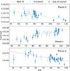 |
Fig. 1 Stellar line contrast as a function of S/N for each night. In-transit and out-of-transit are marked as shaded and clear blue, respectively. Each coloured line corresponds to the best fit to the out-of-transit exposures for each night. |
3.2 Classical RM analysis
We analysed the RM effect on the RVs of each planet using the approximate yet accurate analytic formulas provided by Ohta et al. (2005), which are implemented in the Python package PyAstronomy (Czesla et al. 2019). Ohta et al. (2005) formalism is based on a geometrical approach to describe the RM anomaly and is useful for extracting the information on the projected angle between the planetary orbit axis and the stellar spin axis, λ, and the projected stellar spin velocity, v sin i*, where v and i* represent the star’s rotation velocity and the inclination angle of the stellar rotation axis. The stellar rotation period is known to be Prot = 28.16 ± 3 d for a parent star with a radius of R* = 0.58 ± 0.03 R⊙ (Passegger et al. 2024). In our analysis, we combined the RM formalism with the equation Prot = 2πR*/v to constrain the inclination angle of the stellar spin axis, which would later be used to derive the true planetary obliquities.
We used the planetary ephemeris listed in Table A.1 to convert observing epochs into phases and the detrended and Keplerian-corrected RVs from previous Section 3.1. Additional inputs for the RM model are the following: the linear limb-darkening coefficient (ε), the planet-to-star radius ratio (Rp/R*), the semi-major axis of the planetary orbit in units of the star’s radius (a/R*), and the orbital inclination angle (i). The free parameters in our model are λ, v sin i*, ε, and i*. To find the best fit and constrain the uncertainties associated with the free parameters, we applied a Markov chain Monte Carlo (MCMC) method. We used the emcee package (Foreman-Mackey et al. 2013) to run the MCMC simulations with 34 walkers, 20 000 iterations for the burn-in phase, followed by an additional 30 000 iterations to define the posterior samples. We adopted uninformative priors for the free parameters: projected obliquities (ranging from −120 to 90 deg for GJ 9827 b and c, and from −90 to 90 deg for GJ 9827 d), projected stellar rotation velocity (between 0 and 10 km s−1), the linear limb-darkening coefficient (between 0 and 1), and the star’s rotation axis inclination (between 0 and 180 deg). Additionally, we allowed R*, Prot, Rp/R*, i, and a/R* to vary according to normal distributions centred on the values listed in Table A.1, with widths equal to one standard error to obtain more conservative uncertainty estimates for the free variables during the MCMC process.
We followed two approaches. In the first approach, all three planets were fitted simultaneously (joint-system analysis) by adopting a single v sin i* independently of the planetary obliquities. In the second approach, each planet was studied separately, with three different v sin i* values being obtained, one for each planet. In all the analyses, the linear limb-darkening coefficient was not constrained, obtaining an average value of ε = 0.5 ± 0.3. The other free parameters exhibit posterior distributions with Gaussian-like shapes, suggesting that the MCMC solutions converged to reasonable values. The corner plot depicting the posterior distributions for the joint-system study is given in Figure D.1. Table 2 and Figure 2 present the results and best-fit models from both approaches, including the maximum amplitude of the resulting best-fit RM models. All derived parameters are consistent within the quoted error bars. Note that the stellar v sin i* obtained for GJ 9827 d from the individual analysis suggests that the stellar rotation is moderately lower along the chord described by the path of planet d. However, in the corner plot of this specific analysis there is a strong correlation between the projected rotation velocity and the inclination angle of the stellar spin axis, which is not broken by the RV data alone. This degeneracy is not present in the other two planets of the individual study and the joint-system analysis. The three transiting planets show rather small RM amplitudes, typically below 1 m s−1.
The parent star exhibits a low v sin i*, and its spin axis is nearly perpendicular to the line of sight. Within the 1σ uncertainty, the projected planetary obliquities suggest that all three planets are coplanar and aligned with the stellar spin axis. True planetary obliquities (ψ) were calculated according to the method described in Section 4. Table 2 presents the 3D obliquities derived from the joint-system analysis, as this approach provides a more tightly constrained i*.
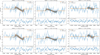 |
Fig. 2 Classical RM analysis for all three planets. The top three panels represent the joint system analysis, while the bottom three panels show the results from the individual planet analysis. The uncertainty of the models is depicted by the shaded grey area. |
3.3 RM revolutions analysis
The information in the disc-integrated CCF is summarised with a single measurement for the classical RM modelling, the RV. In the RM Revolutions analysis, the information contained from the stellar surface occulted by the planet was analysed using the full information contained in the planet-occulted CCF. The planet-occulted CCFs were extracted from the disc-integrated CCFs in a series of steps, detailed below.
At this point, all exposures were aligned in the stellar rest frame. The out-of-transit exposures were co-added to build a master out-of-transit CCF to represent the unocculted star. Each exposure was then scaled to a common relative flux level computed from the master-out CCF. The flux levels of the in-transit exposures were set to a common flux level relative to light curves computed using the batman package (Kreidberg 2015) combined with parameters in table A.1. The planet-occulted CCFs were then computed by subtracting the in-transit exposures from the master-out. The resulting CCFs were then re-scaled to a common flux level, enabling a more direct comparison between the planet-occulted CCFs. These steps allow us to directly trace the stellar surface properties along the transit chord of the planet; for a detailed description, see Bourrier et al. (2021).
Planet-occulted CCFs were analysed individually using MCMC to explore the full parameter space and obtain robust uncertainty estimates. For this, we utilised the Python package emcee (Foreman-Mackey et al. 2013). In this step, the quality and information contained in each CCF was evaluated. For each planet, the ingress and egress exposures were removed, as the CCFs for these exposures show uniform posteriors for at least two of the model parameters or values outside its definition range. These exposures suffers from high noise levels due to the combined effect of partial occultation of the star during the exposure and the faintness of the stellar limb. Since these exposures exhibit faint or no signal while dominated by noise, this further motivates the exclusion of these exposures from the in-transit analysis.
We used a Gaussian model to fit each planet-occulted CCF, consistent with the model applied to the disc-integrated CCFs. Due to the small size of the planets, these CCFs were dominated by noise, making the local stellar line difficult to detect in many exposures. Therefore, we assumed that the Gaussian model remains a suitable approximation. To determine the bestfit parameters, we used MCMC to analyse each exposure with 50 walkers, 1500 steps, and a 500-step burn-in phase. Walkers were initialised over broad ranges for each parameter, with these ranges determined from the best fit parameters observed in the disc-integrated CCF analysis. We used uniform priors for all parameters: U[0,1] for line contrast, U[0,10]kms−1 for FWHM, and U[−4,4]kms−1 for the stellar surface RV. These priors were chosen to ensure comprehensive exploration of the parameter space, with the FWHM prior extending beyond the disc-integrated values (consistently below 6.0 kms−1) and the RV prior encompassing the latest literature value of v sin i < 1.75 km s−1 (Passegger et al. 2024), allowing for broader exploration given the noisy data.
The planet-occulted CCFs are presented in the left column of Figure 3, with planets b, c, and d shown from top to bottom. Each CCF represents the star’s surface velocity on the x axis and the orbital phase on the y axis, and the colour scale represents the normalised and scaled flux. We can see the brighter track at the centre for each planet, which is more evident for planet d and least visible for planet c. However, it can be seen from the middle to the end of the transit. Further, we can see how the track traces the surface velocity from negative to positive values from the start to the end of the transit. The RM Revolutions model is shown in the middle, and residuals from subtracting the best-fit model are shown in the right column, and further explained in Section 3.3.2.
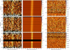 |
Fig. 3 Left column : planet-occulted CCF maps for planets b, c, and d (top to bottom panel), with time (orbital phase) on the y axis and the stellar surface velocity on the x axis. The occulted stellar line is visible as a bright track for each planet, but remains close to the noise level. It is most prominent for planet d. Middle column : best RM Revolutions model for the occulted stellar line during transit. Right column : residual map after subtracting the best RM Revolutions model (middle panel) from the planet-occulted CCFs (left panel). |
3.3.1 Individual planet analysis
Due to the small size of the planets, the individual planet-occulted CCFs exhibit low S/N, causing the local stellar line to be undetected in most exposures. This makes it challenging to constrain the line properties from single exposures alone. To address this, we used the RM Revolutions approach, which leverages information from all in-transit exposures to simultaneously fit a model for the local stellar line across the entire transit. In this model, we used the parameters λ and the equatorial velocity (veq) to model the stellar surface RVs along the transit chord, combined with the line properties, the contrast, and FWHM. We used uniform priors for λ with boundaries set to the definition range U[−180,180]° and for the equatorial velocity we used veq U[0,5] km s−1. We used the same priors for the line contrast and FWHM as used in the individual planet-occulted CCF analysis.
We analysed the line parameters: contrast and FWHM for each planet to search for any spatial correlations along the transit chord. For each transit, we find that a constant value represents these parameters best. Hence, there are no variations during the transit, and a constant value was used to fit the entire transit. The individual analysis of each planet shows varying v sin i*, with planet c resulting in a faster stellar rotation (>4 km s−1), and planet d giving a high probability of slower rotation (< 1 km s−1).
In the final RM Revolutions fit of planet b, 12 in-transit exposures were used. This dataset also shows the largest systematics in the out-of-transit data, making the analysis of the in-transit RV variation difficult; see Figure 2. Further, the two exposures after mid-transit show a large jump from the general trend, both seen as outliers in the disc-integrated RV series and in the planet-occulted stellar surface velocity; see Figure 5. For planet b, we find the values for the parameters v sin i =  km s−1 and λ =
  . For planet c, the smallest planet in the system, we measure a faster stellar rotation, with a derived v sin i =
  km s−1, higher than the value reported by Passegger et al. (2024) (v sin i > 1.75 km s−1), and a measured spin-orbit angle of λ =
  . The comparatively high v sin i* discrepancy is discussed in more detail in Appendix C. For the outer planet, d, the largest planet in the system, the measured stellar rotation and derived rotational velocity are similar to the ones for planet b, with a v sin i =
  km s−1 and a spin-orbit angle of
  . For the individual analysis of planets b and d, we measured slow rotational velocities that are consistent with zero. However, for planet c, we measured a higher rotational velocity. As a next step, we modelled the system jointly by modelling the three transits simultaneously.
3.3.2 Joint-system analysis
In the final step of our analysis, we modelled all planets simultaneously using a total of 41 in-transit exposures: 12 for planet b, 19 for planet c, and 10 for planet d, discarding only ingress and egress exposures for consistency with the individual planet analyses. All transits were modelled with Gaussian line profiles, and the localised stellar line was fitted using the following parameters, the stellar inclination (cos i*), λ, and the stellar rotation period (Prot) to match the RV centroid of the planet-occulted CCFs. Rather than using v sin i*, we adopted Prot along with R* and cos i* to model the stellar surface RVs along the transit chord, allowing us to directly derive the true 3D spin-orbit angle from the sky-projected spin-orbit angle. This approach is further supported by the precise stellar rotation period constraints from Kepler photometry in literature values, making Prot a more reliable parameter to compare for our analysis. Gaussian priors on R* were applied based on the Kepler photometry from Passegger et al. (2024), ensuring consistency with independent stellar constraints.
From the individual analyses, we found that the line properties (contrast and FWHM) for the transits of b and c are similar. Hence, we adopted a single line model for these transits. For the transit of planet d, we find a different contrast and FWHM values; it was therefore assigned independent line parameters. With the large time gap between the observations this likely corresponds to the long-term evolution of the stellar emission. Incorporating these differences into the joint system analysis by simultaneously fitting all exposures enabled us to further constrain v sin i* and to model both the rotation period and stellar inclination. This simultaneous approach provides stronger leverage on the stellar parameters than the individual analyses alone.
We initialised the MCMC walkers around the system parameters obtained from the individual analysis in Sect. 3.3.1, spanning a more than 1σ range. We adopted the same priors as in the individual analyses for all parameters common to both. For the newly introduced parameter, Prot, we used a uniform prior, U[1,40] d, keeping it large enough to encompass slower rotation than literature values (28-29 d) (Rice et al. 2019; Bonomo et al. 2023; Passegger et al. 2024), while enabling and accommodating the higher rotation periods measured in the individual analysis. For cos i*, we employed the full definition range, U[−1,1], and for R*, we applied Gaussian priors with R* = 0.58 ± 0.03 R⊙ from Passegger et al. (2024). The MCMC was run with 30 walkers for 7700 steps, discarding the first 2500 steps as burn-in. The full posterior distribution is presented in Figure D.2.
Our analysis indicates that the star is observed equator-on, with a derived stellar inclination of  . The sky-projected obliquities of the three planets were measured as follows:
  ,
,  , and
, and  , and are consistent with those obtained from the individual planet analyses (see Section 3.3.1).
The inferred v sin i* distribution is broad and bimodal, with a median of 2.26 km s−1, with two modes around 1 km s−1 and 2.5 km s−1. These correspond to stellar rotation periods of 29.3 and 11.7 days, respectively. The higher v sin i* mode appears to be driven primarily by the transit of planet c, which contributes nearly half (46%) of the in-transit exposures. To assess the significance of the planetary signals, we tested a null hypothesis by fitting the model in the continuum which is excluded from any planetary features. This yielded a BIC that was 315 points higher than that of our best-fit model, supporting the detection of planetary signatures.
However, our measured v sin i* values are notably higher than those reported by Passegger et al. (2024), who found values near 1 km s−1 after accounting for both rotational and macroturbulent broadening. Our approach yields a measurement of v sin i* that is independent of these broadening effects, due to the spatial resolution along the transit chord. To address this, we performed an additional fit in which the stellar rotation period was constrained and consistent with the measured photometric rotation period. This allowed us to isolate the lower mode for v sin i* and obtain a stellar rotation rate more in line with values derived from photometric observations.
We used an asymmetric Gaussian distribution as priors for the stellar rotation with Prot =  d, using rotation periods from Kepler data (Passegger et al. 2024). Combined with normal priors for the stellar radius, we have an upper limit for the derived v sin i* , while keeping a common value for all three planets. Again, we find the star to be near equator-on with i* =
  . The best fitting RM model yields sky-plane obliquities for the three planets:
  ,
,  , and
, and  . Hence, the resulting spin-orbit angles for the two cases are unchanged, but with increased uncertainties related to the slower rotation. Further, the BIC values perform 307 points lower than the null hypothesis and 8 points higher than the previous case. We find that all planets are aligned and coplanar within one sigma. For planet b, we still do not constrain the spin-orbit angle. This observation also displays systematics in the RVs in the out-of-transit data; see Figure 2.
Figure 4 shows the average planet-occulted CCFs, aligned using the best-fit model. The corresponding surface radial velocities from the model are displayed in Figure 5, overlaid on the observed RVs derived from the planet-occulted CCFs. For planets c and d, the model reproduces the observed velocities well. In contrast, the in-transit RVs for planet b exhibit significant scatter, which prevents a good fit from being achieved. Nonetheless, a polar orbit is ruled out at the 1σ level. Overall, the model favours a spin-orbit aligned configuration.
4 GJ 9827 system architecture
The stellar inclination was measured to be close to 90°. Therefore, there is no degeneracy between the two stellar configurations, north and south, as the 3D spin-orbit angle is symmetrical with respect to the plane of the sky with i* ≈ 90°. Hence, we computed the spin-orbit angle over the full angular distribution. We derived the 3D spin-orbit angle for the three planets as
 (1)
(1)
The 3D spin-orbit angles were computed by combining the posterior distributions for ip, λ, and i* derived from the Revolutions analysis. For the 3D spin-orbit angle we find moderate misalignments for all three planets: Ψb =  , Ψc =
  , and Ψd =
  . While the posterior distributions extend to moderate misalignments, the 3D spin-orbit angles remain weakly constrained and are consistent with aligned orbits within 2σ.
The posterior distributions for all 3D spin-orbit angles are shown in the top panel of Figure 6, with the median value as a vertical line for each planet. The distributions of the 3D obliquity angles are skewed, largely due to the combination of broad distributions in the input parameters and the non-linear transformation used to compute Ψ. To highlight the skewness introduced by the non-linear transformation from cos(Ψ) to Ψ, both distributions are shown in Figure B.1. This effect introduces an apparent bias toward misaligned orbits in their 3D spin-orbit angle when the sky-projected spin-orbit angle is close to zero, as is further discussed in Appendix B. A similar bias for misaligned systems in their true 3D spin-orbit angles has been reported by Attia et al. (2023).
The mutual inclination between the three orbital planes of planet b, c, and d, is shown in the middle and bottom panels in Figure 6, corresponding to the two possible configurations. This degeneracy arises as we have two possible solutions for the same RM signal; namely, A = (λ & ipl) or B = (-λ & 180° - ipl). Both configurations yield mutual inclinations that are consistent with a coplanar system, and rule out large mutual inclinations between planets (Fig. 7).
The orbital architecture of GJ 9827 is consistent with a coplanar configuration, and rules out large spin-orbit misalignment. However, the measurements are too imprecise to rule out any moderate misalignment definitively. A coplanar system supports the role of disc migration, where planets form and migrate within the protoplanetary disc. Any misalignment between the planetary orbits and the stellar spin axis could arise from a misalignment between the star and the protoplanetary disc. However, additional observations are required to better constrain the spin-orbit angles and rule out smaller misalignments between the planets. The system’s near-resonant orbits provide additional support for a smooth and slow disc migration, where planets migrate together, while maintaining their initial coplanarity.
Disc-driven migration is expected to result in planetary orbits that are well aligned with the stellar equator (Winn & Fabrycky 2015), as significant misalignments between the protoplanetary disc and the stellar spin axis are not generally anticipated. However, if the disc were initially tilted relative to the stellar rotation, some degree of spin-orbit misalignment could arise. For strongly misaligned systems, high-eccentricity tidal migration is believed to be the primary cause, as it does not retain any memory of the initial orientation (Naoz et al. 2012; Albrecht et al. 2012; Nelson et al. 2017). The 3D spin-orbit angles in this work suggest that the planets have retained their coplanarity, but do not rule out a moderate misalignment between the stellar spin axis and the orbital planes of the planets. Such a misalignment could result from an initially tilted protoplanetary disc. To distinguish between these scenarios and confirm or reject a moderate spinorbit misalignment, future observations of this system will be necessary.
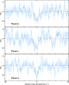 |
Fig. 4 Average CCF from planet-occulted profiles along the transit chord aligned with the best-fit Revolutions model. The same flux scale is used for all three planets. Best Gaussian fits are shown as dashed black lines. |
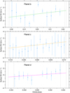 |
Fig. 5 Stellar surface RVs of the occulted region during transit for each planet with orbital phase on the x axis. The surface RV retrieved from the best-fit RM revolutions model is overlaid as a solid line for each planet. Transit contacts are shown as vertical grey lines. |
5 Conclusions
We conducted a simultaneous analysis of three transiting planets in the system GJ 9827, observed with ESPRESSO. Our findings suggest that the system is coplanar within the uncertainties for both the sky-projected and 3D spin-orbit angles. The sky-projected spin-orbit angles indicate that all three planets are aligned with the stellar spin. These results are consistent across both methods used: the classical RM and the Revolutions technique.
The inferred 3D spin-orbit angles are consistent with a coplanar system architecture and rule out large misalignments between the planetary orbits and the stellar spin axis. The two inner planets exhibit larger misalignments, although they remain within 10 deg of each other. For the outermost planet, planet d, the misalignment is smaller but still consistent with a coplanar configuration for the three planets. The 3D spin-orbit angles extend to moderate misalignments for all planets; however, they are all aligned with the stellar spin axis within a 2 σ interval. The coplanarity of the system supports a scenario of smooth, disc-driven, and convergent migration for this compact multiplanet system. The shared misalignment of these planets could be explained by a primordial tilt between the stellar spin axis and the protoplanetary disc. However, further observations are required to confirm this and to place tighter constraints on the system’s spin-orbit architecture.
To date, measurements of the spin-orbit angle in compact, near-resonant multi-planet systems are rare. Prior to this work, only the TRAPPIST-1 system, composed of Earth- and super-Earth-sized planets, has had sky-projected spin-orbit measurements for more than one planet, with planets b, e, and f found to be coplanar and aligned with the host star (Hirano et al. 2020). GJ 9827 is therefore the second such system with multiple spin-orbit angle measurements. Additional studies of individual planets in compact near-resonant systems, namely Kepler-9 b (Wang et al. 2018) and HD110067c (Zak et al. 2024), have also found the sky-projected obliquities to be consistent with alignment. Together, these results support the idea of smooth, convergent disc-driven migration as the dominant dynamical pathway for this class of systems.
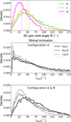 |
Fig. 6 Top panel : posterior distributions for the 3D spin-orbit angle derived for each planet, with the median values indicated by vertical lines. Middle panel : mutual inclination distributions for all three planet pairs assuming configuration A as the spin-orbit geometry for each planet. Bottom panel : mutual inclination distributions for mixed configurations, whereby each planet adopts either configuration A or B. |
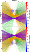 |
Fig. 7 Projection of GJ 9827 on the sky plane is shown as viewed equator-on. The black arrow indicates the direction of the stellar spin axis, while the black line traces the stellar equator. The orbital plane normals of the three planets are indicated by the coloured arrows: green for planet b, orange for c, and purple for d. The stellar surface is colour-coded according to the projected radial surface velocity. The solid lines indicate the best-fit orbits for each planet, while the shaded lines illustrate randomly drawn orbits from each distribution of the semi-major axis, orbital inclination, and spin-orbit angle. |
Acknowledgements
This work has been carried out in the frame of the National Centre for Competence in Research PlanetS supported by the Swiss National Science Foundation (SNSF). This project has received funding from the European Research Council (ERC) under the European Union’s Horizon 2020 research and innovation programme (project SPICE DUNE, grant agreement No 947634). The INAF authors acknowledge financial support of the Italian Ministry of Education, University, and Research with PRIN 201278X4FL and the ’Progetti Premiali’ funding scheme. This work was financed by Portuguese funds through FCT (Fundaçâo para a Ciência e a Tecnologia) in the framework of the project 2022.04048.PTDC (Phi in the Sky, DOI 10.54499/2022.04048.PTDC). CJM also acknowledges FCT and POCH/FSE (EC) support through Investigador FCT Contract 2021.01214.CEECIND/CP1658/CT0001 (DOI 10.54499/2021.01214.CEECIND/CP1658/CT0001). JIGH, ASM, RR and CAP acknowledge financial support from the Spanish Ministry of Science, Innovation and Universities (MICIU) projects PID2020-117493GB-I00 and PID2023-149982NB-I00. Co-funded by the European Union (ERC, FIERCE, 101052347). Views and opinions expressed are however those of the author(s) only and do not necessarily reflect those of the European Union or the European Research Council. Neither the European Union nor the granting authority can be held responsible for them. This work was supported by FCT -Fundaçâo para a Ciência e a Tecnologia through national funds by these grants: UIDB/04434/2020 DOI: 10.54499/UIDB/04434/2020, UIDP/04434/2020 DOI: 10.54499/UIDP/04434/2020. FPE and CLO would like to acknowledge the Swiss National Science Foundation (SNSF) for supporting research with ESPRESSO through the SNSF grants nr. 140649, 152721, 166227, 184618 and 215190. The ESPRESSO Instrument Project was partially funded through SNSF’s FLARE Programme for large infrastructures. We acknowledge financial support from the Agencia Estatal de Investigación of the Ministerio de Ciencia e Innovación MCIN/AEI/10.13039/501100011033 and the ERDF “A way of making Europe” through project PID2021-125627OB-C32, and from the Centre of Excellence “Severo Ochoa” award to the Instituto de Astrofisica de Canarias. SNSF Postdoctoral Fellow R.A. acknowledges the Swiss National Science Foundation (SNSF) support under the Post-Doc Mobility grant P500PT_222212 and the support of the Institut Trottier de Recherche sur les Exoplanètes (IREx).
References
- Albrecht, S., Winn, J. N., Johnson, J. A., et al. 2012, ApJ, 757, 18 [NASA ADS] [CrossRef] [Google Scholar]
- Attia, M., Bourrier, V., Delisle, J. B., & Eggenberger, P. 2023, A&A, 674, A120 [NASA ADS] [CrossRef] [EDP Sciences] [Google Scholar]
- Bate, M. R., Lodato, G., & Pringle, J. E. 2010, MNRAS, 401, 1505 [NASA ADS] [CrossRef] [Google Scholar]
- Batygin, K. 2012, Nature, 491, 418 [NASA ADS] [CrossRef] [Google Scholar]
- Bonomo, A. S., Dumusque, X., Massa, A., et al. 2023, A&A, 677, A33 [NASA ADS] [CrossRef] [EDP Sciences] [Google Scholar]
- Bouchy, F., Pepe, F., & Queloz, D. 2001, A&A, 374, 733 [NASA ADS] [CrossRef] [EDP Sciences] [Google Scholar]
- Bourrier, V., Lovis, C., Cretignier, M., et al. 2021, A&A, 654, A152 [NASA ADS] [CrossRef] [EDP Sciences] [Google Scholar]
- Bourrier, V., Delisle, J.-B., Lovis, C., et al. 2024, A&A, 691, A113 [NASA ADS] [CrossRef] [EDP Sciences] [Google Scholar]
- Chatterjee, S., Ford, E. B., Matsumura, S., & Rasio, F. A. 2008, ApJ, 686, 580 [NASA ADS] [CrossRef] [Google Scholar]
- Czesla, S., Schröter, S., Schneider, C. P., et al. 2019, PyA: Python astronomy-related packages [Google Scholar]
- Dressing, C. D., Hardegree-Ullman, K., Schlieder, J. E., et al. 2019, VizieR Online Data Catalog: 86 cool dwarfs observed during K2 Campaigns 117 (Dressing+, 2019), VizieR On-line Data Catalog: J/AJ/158/87. Originally published in: 2019AJ....158...87D [Google Scholar]
- Fabrycky, D., & Tremaine, S. 2007, ApJ, 669, 1298 [NASA ADS] [CrossRef] [Google Scholar]
- Fielding, D. B., McKee, C. F., Socrates, A., Cunningham, A. J., & Klein, R. I. 2015, MNRAS, 450, 3306 [NASA ADS] [CrossRef] [Google Scholar]
- Foreman-Mackey, D., Hogg, D. W., Lang, D., & Goodman, J. 2013, PASP, 125, 306 [Google Scholar]
- Fulton, B. J., Petigura, E. A., Howard, A. W., et al. 2017, AJ, 154, 109 [Google Scholar]
- Gaia Collaboration (Vallenari, A., et al.) 2023, A&A, 674, A1 [NASA ADS] [CrossRef] [EDP Sciences] [Google Scholar]
- Hirano, T., Gaidos, E., Winn, J. N., et al. 2020, ApJ, 890, L27 [NASA ADS] [CrossRef] [Google Scholar]
- Kass, R. E., & Raftery, A. E. 1995, J. Am. Statist. Assoc., 90, 773 [CrossRef] [Google Scholar]
- Kreidberg, L. 2015, PASP, 127, 1161 [Google Scholar]
- Lai, D. 2014, MNRAS, 440, 3532 [NASA ADS] [CrossRef] [Google Scholar]
- Lai, D., Foucart, F., & Lin, D. N. C. 2011, MNRAS, 412, 2790 [NASA ADS] [CrossRef] [Google Scholar]
- Liddle, A. R. 2007, MNRAS, 377, L74 [NASA ADS] [Google Scholar]
- McLaughlin, D. B. 1924, ApJ, 60, 22 [Google Scholar]
- Naoz, S., Farr, W. M., & Rasio, F. A. 2012, ApJ, 754, L36 [NASA ADS] [CrossRef] [Google Scholar]
- Nelson, B. E., Ford, E. B., & Rasio, F. A. 2017, AJ, 154, 106 [NASA ADS] [CrossRef] [Google Scholar]
- Niraula, P., Redfield, S., Dai, F., et al. 2017, AJ, 154, 266 [Google Scholar]
- Ohta, Y., Taruya, A., & Suto, Y. 2005, ApJ, 622, 1118 [Google Scholar]
- Passegger, V. M., Suárez Mascareño, A., Allart, R., et al. 2024, A&A, 684, A22 [NASA ADS] [CrossRef] [EDP Sciences] [Google Scholar]
- Pepe, F., Cristiani, S., Rebolo, R., et al. 2021, A&A, 645, A96 [NASA ADS] [CrossRef] [EDP Sciences] [Google Scholar]
- Piaulet-Ghorayeb, C., Benneke, B., Radica, M., et al. 2024, ApJ, 974, L10 [NASA ADS] [CrossRef] [Google Scholar]
- Rice, K., Malavolta, L., Mayo, A., et al. 2019, MNRAS, 484, 3731 [NASA ADS] [CrossRef] [Google Scholar]
- Rodriguez, J. E., Vanderburg, A., Eastman, J. D., et al. 2018, AJ, 155, 72 [NASA ADS] [CrossRef] [Google Scholar]
- Rossiter, R. A. 1924, ApJ, 60, 15 [Google Scholar]
- Schwarz, G. 1978, Ann. Statist., 6, 461 [Google Scholar]
- Teyssandier, J., Terquem, C., & Papaloizou, J. C. B. 2013, MNRAS, 428, 658 [NASA ADS] [CrossRef] [Google Scholar]
- Wang, S., Addison, B., Fischer, D. A., et al. 2018, AJ, 155, 70 [Google Scholar]
- Winn, J. N., & Fabrycky, D. C. 2015, ARA&A, 53, 409 [NASA ADS] [CrossRef] [Google Scholar]
- Wu, Y., & Murray, N. 2003, ApJ, 589, 605 [Google Scholar]
- Zacharias, N., Finch, C. T., Girard, T. M., et al. 2012, VizieR Online Data Catalog: UCAC4 Catalogue (Zacharias+, 2012), VizieR On-line Data Catalog: I/322A. Originally published in: 2012yCat.1322....0Z; 2013AJ....145...44Z [Google Scholar]
- Zak, J., Boffin, H. M. J., Sedaghati, E., et al. 2024, A&A, 687, L2 [NASA ADS] [CrossRef] [EDP Sciences] [Google Scholar]
- Zanazzi, J. J., & Lai, D. 2018, MNRAS, 478, 835 [NASA ADS] [CrossRef] [Google Scholar]
Appendix A System properties
System parameters used and derived in the analysis of GJ 9827.
Appendix B 3D spin-orbit angle transformation
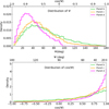 |
Fig. B.1 Top panel: distribution of Ψ, with the top axis showing the corresponding cos(Ψ) values. Green, orange, and magenta curves corresponds to planet b, c, and d, respectively. Bottom panel: distribution of cos(Ψ) values before the trigonometric transformation, with the bottom axis showing cos(Ψ) and the top axis mapped to Ψ. The sharp contrast-between the two panels illustrate the non-linearity near the aligned case (0°). |
To interpret the distributions of the sky-projected spin-orbit angles, the inclination of the stellar spin axis, and the resulting 3D spin-orbit angles, the Ψ and cos(Ψ) distributions are shown in Figure B.1. The skewness of the Ψ distributions is clearly illustrated by the transformation from cos(Ψ) to Ψ, which is strongly non-linear towards the aligned case: even a small shift in cos(Ψ) results in a large change in Ψ.
This introduces an important caveat when computing the 3D spin-orbit angle near alignment. A broader distribution in either λ, i*, or both, can produce a skewed Ψ distribution, shifting the sky-projected alignment towards larger 3D spin-orbit angles. This effect can bias the interpretation of systems that are intrinsically well aligned. Hence, this highlights the limitations of deriving the 3D spin-orbit angle with high precision, especially when the uncertainties in the projected spin-orbit angle and the stellar inclination are large.
To visualise the 3D spin-orbit geometry, Figure B.2 shows the probability distribution of the 3D spin-orbit angle for planet d, projected onto the sky plane (top) and in a pole-on view (bottom). These visualisations illustrate the probability density of allowed spin-orbit orientations, highlighting the very low probability near the perfect alignment.
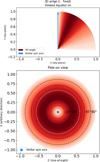 |
Fig. B.2 Probability distribution for Ψd, computed as a density function from posterior samples. Top panel: equator-on view, showing the probability projected onto the sky plane. Bottom panel: pole-on view, constructed assumed spherical symmetry around the stellar spin axis. Darker colours indicate higher probability. Dashed black lines show angular separations from the stellar spin axis for visual reference, and the white dashed line marks the median value (33°. Since Ψ is an absolute angle, orientations in the bottom panels are directionally degenerate. |
Appendix C Planet C CCF analysis
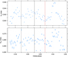 |
Fig. C.1 Hα and R′HK as a function of orbital phase. The grey vertical lines mark the transit contacts, and the red vertical line marks the cut applied before excluding exposures identified as a potential flaring event, most clearly visible in Hα. |
Several stellar activity indicators were analysed for all three transits. An emission feature is identified during the transit of planet c on the night 2022-08-07 in Hα, and is also observed in other indicators such as R′HK; see Figure C.1. As the out-oftransit baseline immediately before and after the transit does not deviate for planet c, the last 28 exposures were excluded from the analysis. These are marked by a red line in Figure C.1.
No significant deviations are observed in the line properties shown in Figure C.2, except for the last two exposures, which display a clear drop in contrast. However, this is likely due to observing conditions at the end of night rather than stellar activity related. As discussed in Section ??, the analysis of the transit of planet c yields a higher v sin i* compared to planets b and d, as well as to literature values. Extending the baseline to include the full dataset results in a similar v sin i*, indicating that the shorter baseline for this transit does not have a significant impact on the results.
From the analysis of the disc-integrated CCF properties, we do not find any clear discrepancies leading to the high v sin i* derived for planet c. Further, when analysing the surface RVs derived directly from the planet-occulted CCFs, we find a lower v sin i* compared to the full Revolutions model, in which the entire spectral line is modelled during the transit. This may indicate variations in the spectral line shape along the transit chord that are not fully captured in the analysis. In particular, the small planetary size leads to a low S/N in the planet-occulted profiles, which limit our ability to resolve such variations, possibly leading to biases when assuming a fixed Gaussian line shape derived from the disc-integrated analysis.
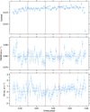 |
Fig. C.2 Same as Figure C.1, but for the line properties contrast, FWHM, and RV residuals. There’s no clear deviations in any of the line properties after the exclusion of exposures. |
Appendix D Posterior distribution
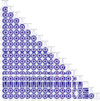 |
Fig. D.1 Distribution of the posteriors for the Classical analysis of the RM effect (joint-system approach). |
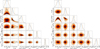 |
Fig. D.2 Posterior distribution of selected parameters from the joint Revolutions analysis. The left corner plot shows the results using uniform priors on Prot. The right plot shows the final joint fit using normal priors on Prot. |
All Tables
All Figures
|
Fig. 1 Stellar line contrast as a function of S/N for each night. In-transit and out-of-transit are marked as shaded and clear blue, respectively. Each coloured line corresponds to the best fit to the out-of-transit exposures for each night. |
| In the text | |
|
Fig. 2 Classical RM analysis for all three planets. The top three panels represent the joint system analysis, while the bottom three panels show the results from the individual planet analysis. The uncertainty of the models is depicted by the shaded grey area. |
| In the text | |
|
Fig. 3 Left column : planet-occulted CCF maps for planets b, c, and d (top to bottom panel), with time (orbital phase) on the y axis and the stellar surface velocity on the x axis. The occulted stellar line is visible as a bright track for each planet, but remains close to the noise level. It is most prominent for planet d. Middle column : best RM Revolutions model for the occulted stellar line during transit. Right column : residual map after subtracting the best RM Revolutions model (middle panel) from the planet-occulted CCFs (left panel). |
| In the text | |
|
Fig. 4 Average CCF from planet-occulted profiles along the transit chord aligned with the best-fit Revolutions model. The same flux scale is used for all three planets. Best Gaussian fits are shown as dashed black lines. |
| In the text | |
|
Fig. 5 Stellar surface RVs of the occulted region during transit for each planet with orbital phase on the x axis. The surface RV retrieved from the best-fit RM revolutions model is overlaid as a solid line for each planet. Transit contacts are shown as vertical grey lines. |
| In the text | |
|
Fig. 6 Top panel : posterior distributions for the 3D spin-orbit angle derived for each planet, with the median values indicated by vertical lines. Middle panel : mutual inclination distributions for all three planet pairs assuming configuration A as the spin-orbit geometry for each planet. Bottom panel : mutual inclination distributions for mixed configurations, whereby each planet adopts either configuration A or B. |
| In the text | |
|
Fig. 7 Projection of GJ 9827 on the sky plane is shown as viewed equator-on. The black arrow indicates the direction of the stellar spin axis, while the black line traces the stellar equator. The orbital plane normals of the three planets are indicated by the coloured arrows: green for planet b, orange for c, and purple for d. The stellar surface is colour-coded according to the projected radial surface velocity. The solid lines indicate the best-fit orbits for each planet, while the shaded lines illustrate randomly drawn orbits from each distribution of the semi-major axis, orbital inclination, and spin-orbit angle. |
| In the text | |
|
Fig. B.1 Top panel: distribution of Ψ, with the top axis showing the corresponding cos(Ψ) values. Green, orange, and magenta curves corresponds to planet b, c, and d, respectively. Bottom panel: distribution of cos(Ψ) values before the trigonometric transformation, with the bottom axis showing cos(Ψ) and the top axis mapped to Ψ. The sharp contrast-between the two panels illustrate the non-linearity near the aligned case (0°). |
| In the text | |
|
Fig. B.2 Probability distribution for Ψd, computed as a density function from posterior samples. Top panel: equator-on view, showing the probability projected onto the sky plane. Bottom panel: pole-on view, constructed assumed spherical symmetry around the stellar spin axis. Darker colours indicate higher probability. Dashed black lines show angular separations from the stellar spin axis for visual reference, and the white dashed line marks the median value (33°. Since Ψ is an absolute angle, orientations in the bottom panels are directionally degenerate. |
| In the text | |
|
Fig. C.1 Hα and R′HK as a function of orbital phase. The grey vertical lines mark the transit contacts, and the red vertical line marks the cut applied before excluding exposures identified as a potential flaring event, most clearly visible in Hα. |
| In the text | |
|
Fig. C.2 Same as Figure C.1, but for the line properties contrast, FWHM, and RV residuals. There’s no clear deviations in any of the line properties after the exclusion of exposures. |
| In the text | |
|
Fig. D.1 Distribution of the posteriors for the Classical analysis of the RM effect (joint-system approach). |
| In the text | |
|
Fig. D.2 Posterior distribution of selected parameters from the joint Revolutions analysis. The left corner plot shows the results using uniform priors on Prot. The right plot shows the final joint fit using normal priors on Prot. |
| In the text | |
Current usage metrics show cumulative count of Article Views (full-text article views including HTML views, PDF and ePub downloads, according to the available data) and Abstracts Views on Vision4Press platform.
Data correspond to usage on the plateform after 2015. The current usage metrics is available 48-96 hours after online publication and is updated daily on week days.
Initial download of the metrics may take a while.