| Issue |
A&A
Volume 584, December 2015
|
|
|---|---|---|
| Article Number | A51 | |
| Number of page(s) | 16 | |
| Section | Interstellar and circumstellar matter | |
| DOI | https://doi.org/10.1051/0004-6361/201425583 | |
| Published online | 18 November 2015 | |
Online material
Appendix A: Optical magnitudes during the HST observations
The evolution of the optical magnitude between the two HST observations is required to check if particular absorber properties are reasonable, e.g., if they provide a sufficient amount of V band extinction.
For the 2011 HST observation, we use the STIS acquisition images obtained just prior to the COS observations to estimate the optical brightness assuming an effective temperature of 4000 K and AV = 0.78 as found by Bouvier et al. (2013) for the bright state. We find a V-magnitude of about 13.5which is consistent with a short HST STIS G430L spectrum preceding the COS exposures (the G430L partly overlaps with the V bandpass). This magnitude is typical for the bright state of AA Tau and indicates some absorption by the inner disk warp, because the brightness of the uneclipsed state has been about 12.5 in the V-band.
For the 2013 HST observation, no preceding optical acquisition images nor optical spectra are available so that we estimate the V-magnitude from contemporary optical data points6 (Bouvier et al. 2013). They indicate V ≈ 15 mag, i.e., about 1.5 mag lower than during the previous COS observations.
Appendix B: Period analysis
Figure B.1 shows phased optical light curves of AA Tau.
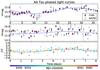 |
Fig. B.1
Phased optical light curves. The color coding in the bottom panel indicates the observing time as encoded in the colorbar. |
| Open with DEXTER | |
Appendix C: FUV continuum evolution
The broad wavelength coverage of the HST COS spectra allows us to determine the wavelength dependent evolution of the FUV continuum flux which, in the simplest scenario, constrains the dust population of the extra absorber. However, additional processes like grain growth, scattering and a non-stellar origin of the FUV continuum hamper direct conclusions and, in fact, none of these three mechanisms can be strictly ruled out.
Appendix C.1: Grain growth
Adding extra extinction cannot cause the continuum to appear bluer in 2013 than in 2011. However, replacing part of the absorber present in 2011 with an absorber that contains on average larger grains causes a bluer continuum. Specifically, replacing ISM-like absorption with AV = 0.4 mag by an absorber with AV = 1.9 and RV = 7 in the Cardelli et al. (1989) description provides a reasonable description of the flux evolution and is compatible with the evolution of the V magnitudes between both epochs (see Appendix A for the evolution of the V magnitudes between both epochs and Fig. 8 (bottom) for the expected continuum flux evolution).
As we have a better data coverage for the time around the XMM-Newton observation, we checked if adding further 0.6 mag of optical extinction with RV = 7 in the Cardelli et al. (1989) description provides a reasonable description of the flux evolution between the bright state and the dim state around the XMM-Newton observation and found that this, again, requires the brighter NIR fluxes contrary to the observations (see discussion of the grain growth scenario in Sect. 5.2). It is impossible to bring the lower NIR fluxes in agreement with the XMM-Newton optical/NUV fluxes by replacing part of an ISM-like absorber during the bright state with an absorber with RV> 3.1 for the 2013 observation. Thus, scattering in the optical is still required to achieve agreement with the lower NIR fluxes when replacing part of the 2011 absorber with an RV> 3.1 one in 2013. Explaining the FUV continuum evolution (moderate flux decrease and blueing) with a modification of the absorber therefore requires scattering in the optical but not in the FUV. In addition, this scenario requires a different explanation for the evolution of the red shifted atomic FUV emission lines which decrease more strongly than the surrounding continuum.
Appendix C.2: Scattering
Scattering can easily explain the blueing of the continuum by postulating that the shortest wavelength already contained scattered photons in 2011 while this did not apply to the same extent to the longer wavelengths. Removing (part of) the direct emission then causes a flux drop as well as a bluer appearance of the continuum. This is compatible with scattering in the optical, but does not explain that the red shifted atomic emission drops more strongly.
Appendix C.3: A non-stellar origin
The analysis of the H2 emission lines showed that the increased absorption mainly affects the line of sight towards the star while, e.g., emission from the outer disk remained largely unaffected. In particular, the high velocity H2 emission reduces by about the same fraction as the FUV continuum suggesting that the FUV continuum originates also within the inner few au of the disk. However, the blueing of the continuum remains unexplained in this scenario; potentially scattering also contributes to the continuum even if its origin is not close to the stellar surface or the shape of the non-stellar emission depends on the distance to the star with redder emission predominately emitted at smaller radii. This is compatible with the evolution of the emission bump at 1600 Å seen in both epochs. This bump has been interpreted in terms of a H2 molecular dissociation quasi-continuum generated by collisions with non-thermal electrons (e.g., Herczeg et al. 2004; Ingleby et al. 2009), i.e., clearly non-stellar. Its flux reduced similarly as the surrounding continuum suggesting that the bump and the majority of the continuum probably experience similar extinction and, thus, probably have a similar spatial origin, too.
To summarize, a non-stellar origin of the FUV continuum is compatible with the observational constrains and scattering might contribute as well while the grain growth scenario appears less likely.
Appendix D: FUV emission lines
The atomic FUV emission lines are usually assumed to be emitted close to the stellar surface and, thus, should experience the same absorption as the photospheric emission. Furthermore, the effect of extinction is more pronounced in the FUV than in the optical. Therefore, we investigate the evolution of the atomic FUV emission lines and concentrate our analysis on the strongest lines (C iv λλ 1548, 1551, N v λλ 1238, 1242 and He iiλ 1640).
Appendix D.1: Details of the data analysis
We removed the H2 “contamination” from the atomic emission lines using the approach presented by France et al. (2014b), i.e., by fitting the wavelength region under consideration with a number of Gaussians convolved with the instrumental line profile and removing components identified as strong H2 fluorescence lines. Lastly, we split the lines into a blue and red shifted part, because shock heated gas within the jet can increase the observed blue shifted emission (e.g., C iv in the DG Tau jet, see Schneider et al. 2013). Further, we exclude velocities with | v | < 50 km s-1 as the COS wavelength calibration is not accurate to within a few 10 km s-1.
COS does not observe these lines simultaneously so that time variability during the observations can influence the results when comparing data from different wavelength settings. Indeed, there is minor variability during the 2011 observations with a slight drop of the C iv and N v count-rates over several hours which could change the C iv to N v ratio by about 20% assuming a continuous, linear evolution. In 2013, the rates remain relatively constant (<10% changes). In the following we neglect these effects, because the variability between the two epochs is much larger.
Appendix D.2: Results
Figure D.1 shows the atomic emission lines and their line fluxes are listed in Table D.1 (which also includes the properties of the C ii and O iii] lines). The red and blue shifted emission evolve differently between both epochs with the red shifted part reducing more strongly than the blue shifted one. This might be due to the fact that red shifted emission should be dominated by emission related to the accretion process (accretion funnels or spots) while the blue shifted emission contains a higher fraction of jet/outflow emission which originates above the disk and is, thus, not subject to the extra absorption. For both red and blue shifted emission, the real flux drop might be higher than observed due to scattered photons. In addition, the red line wing might be “contaminated” by broad, slightly blue-shifted emission lines from the outflow/jet. Furthermore, the atomic emission lines in the FUV are time variable so that tight constrains on the properties of the absorber cannot be derived. With these caveats in mind, we describe the evolution of the red and blue shifted emission separately in the following.
Line fluxes for selected atomic lines and continuum.
|
Fig. D.1
Comparison of the blue and red members of the N v and C iv doublets as well as the evolution of the He ii line. The red members have been scaled by a factor of two to easily see the optical depth effects. The relevant parts of the lines are drawn with thick lines and errors. |
|
| Open with DEXTER | |
Appendix D.2.1: Red shifted emission
The red shifted wings of all atomic emission lines have lower fluxes during the 2013 observation compared to 2011. The fluxes in the red wings of C iv and He ii decrease much more strongly than the N v flux (see sum/red wing in Table D.1) and more strongly than the FUV continuum. The different evolution of C iv and N v fluxes is unexpected, because both species trace rather similar plasma temperatures (log T ~ 5.0 and 5.3) and are usually well correlated (Yang et al. 2012; Ardila et al. 2013). The N v to C iv ratio is closer to the CTTS correlation (Ardila et al. 2013) in 2013 than in 2011. This suggests that the observed N v flux was unusually low in 2011. Because the N v flux was already low in 2011, its factional decrease was less than for the other FUV emission lines. We therefore concentrate on C iv and He ii in the following.
Extinction values (AV) for red shifted FUV emission lines.
Table D.2 summarizes the absorption required to explain the flux evolution for different descriptions of the FUV extinction assuming no intrinsic variability. It shows that the evolution is compatible with ISM-like absorption based on the evolution of the V magnitude, but incompatible with the evolution of the NIR magnitudes which, unfortunately, have not been obtained simultaneously. The evolution is also compatible with an additional RV = 7 absorber. In addition, it is possible to replace part of an ISM-like absorber in 2011 by an RV = 7 absorber assuming scattering contributes to the observed optical but not to the FUV fluxes since this is still compatible with the range of observed NIR magnitudes. Given potential intrinsic time variability, the FUV emission lines are compatible with the different absorber properties discussed above. Furthermore, they are even compatible with higher AV values for an ISM-like absorber assuming that scattering operates also on the atomic FUV emission lines or emission in the red shifted wing of a blue shifted emission component contributes to the red shifted velocity range.
Appendix D.3: Blue shifted atomic emission
The evolution of the blue line wings of the atomic emission lines is visualized in Fig. 8. The blue wings decrease similarly as the surrounding FUV continuum. This suggests that both components are similarly affected by the extra absorber, i.e., less strongly than the red shifted emission originating close to the stellar surface.
Interpreting the continuum emission in terms of a non-stellar origin easily reconciles the evolution of the blue shifted atomic emission lines as they probably originate partly in the outflow/jet, i.e., above the disk. In particular, the C iv emission in 2013 appears slightly blue shifted and rather Gaussian shaped as expected for an outflow/jet origin. Whether the observed atomic emission traces knots within the jet as in DG Tau (Schneider et al. 2013) or a hot stellar wind remains undecided. The similar evolution of blue shifted atomic emission lines and continuum favors a similar spatial origin. Knots within the jet further away from the source would not be affected by the extra absorber, so that an origin close to the disk is likely which favors a stellar wind as the origin of the blue shifted emission lines.
Appendix E: CO emission
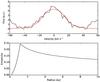 |
Fig. E.1
Top: fit to the 2013 CO emission. Bottom: emissivity of the disk. |
| Open with DEXTER | |
Fluorescent CO emission traces the coolest FUV-emitting plasma observed in our COS spectra. With a typical temperature of a few hundred K it is significantly colder than the observed H2 emission (about 2−3 × 10³ K, France et al. 2011). The flux of the strong CO emission lines is constant indicating that the CO emitting region is not significantly affected by the extra absorber and that the pumping radiation field did not change significantly between the two FUV observations.
In principle, we could also apply the disk emission modeling to the CO emission as we use for the H2 lines. Unfortunately, this is only possible with some accuracy for the CO data from 2013 but not for 2011. Figure E.1 shows that the CO disk emissivity peaks at slightly larger radii than the H2 disk emissivity (CO: 1.2 au, H2: 0.6−0.8 au), but appears in general rather similar to the H2 models for 2013. Therefore, the CO emission comes from similar regions within the disk as the H2 in 2013. Since the total flux did not change significantly, a similar spatial origin in 2011 is likely. This again indicates that only the disk emission within one to two au is affected by the extra absorber.
Appendix F: CO absorption
Figure F.1 shows the evolution of the CO absorption seen in COS. To compare the CO absorption between both epochs, we fit the continuum data (see Appendix C) around the CO absorption bands with a first order polynomial excluding the data falling into the wavelengths ranges of the 1−0 to 4−0 absorption bands. Using this continuum, we calculate an “equivalent width” (EW) of the CO absorption by summing the wavelengths regions unaffected by H2 emission and find that the EW decreases by about 10–21% between both epochs (1 σ confidence range). Including the uncertainty in the continuum level which we assume to be about 10 and 15% for the 2011 and 2013 data, the EW ratio between both epochs is 1.16 ± 0.40. Thus, the CO absorption column densities are similar unless the Doppler broadening parameter b differs significantly between both epochs. Unfortunately, b is not well constrained due to the large instrumental line width (17 km s-1) compared to the b value which is usually around 1 km s-1 (McJunkin et al. 2013). Nevertheless, we attempted to fit the CO absorption using the methods of McJunkin et al. (2013) and find a best fit CO column density of 2.5 × 1018cm-2, a temperature of 100 K and a Doppler b value of 0.5 km s-1 for the 2013 data. This column density is about an order of magnitude higher than that derived by France et al. (2012a) for the 2011 observation, which is mainly caused by the lower b value (0.5 vs. 1.2 km s-1), but also by the much cooler temperature (100 vs. 500 K). However, the errors on the CO column densities are about 1 dex. In summary, we find no significant increase of the CO absorption column density.
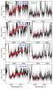 |
Fig. F.1
CO absorption bands with fits. |
| Open with DEXTER | |
While working on the revised version of this paper, Zhang et al. (2015) published CO mid-IR data of AA Tau during the dim state. They find N12CO = 3.2 × 1018 cm-2, which is close to our best fit value from the FUV CO absorption. However, their temperature and broadening values (T ≈ 494 K and 2.2 km s-1, resp.) differ significantly from our absorption model. Adopting their higher broadening value, would strongly decrease the column density required to explain the FUV CO absorption. We thus conclude that both measurements might not trace the same absorber. Given that scattering might contribute to the observed FUV emission, one possibility is that the FUV absorption traces CO located at higher disk altitudes than the MIR CO absorption that is unaffected by scattering.
Using the canonical CO to H ratio of 10-4, Zhang et al. (2015) estimate NH> 3.2 × 1022 cm-2 for the extra absorber, which is of the same order of magnitude as our column density derived from the X-ray data. However, their lower limit is incompatible with the X-ray data. Using the minimum column density absorbed in 2003 (NH = 0.9 × 1022 cm-2) plus their minimum column density (NH = 3.2 × 1022 cm-2) for the extra absorber results in NH> 4.1 × 1022cm-2, but models with NH = 4.1 × 1022 cm-2 do not provide an acceptable fit to the X-ray data. They result in χ2 = 86 (51 d.o.f.) using the Anders & Grevesse (1989) abundances and in χ2 = 78 using the Asplund et al. (2009) abundances, respectively. The best fitting model has χ2 = 33/34.5 (Anders & Grevesse 1989, Asplund et al. 2009 abundances, resp.). The 90% confidence range upper limit on the absorbing column density from the X-ray data is 2.3 × 1022 cm-2 (Anders & Grevesse 1989) and 3.3 × 1022 cm-2 (Asplund et al. 2009).
Appendix G: Additional H2 information
Table G.1 lists the properties of the detected H2 progressions. Figure G.1 shows the evolution of the flux and width of the H2 lines.
Properties of the molecular hydrogen progressions during the two epochs.
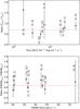 |
Fig. G.1
Evolution of the H2 flux and FWHM for different progressions. |
| Open with DEXTER | |
© ESO, 2015
Current usage metrics show cumulative count of Article Views (full-text article views including HTML views, PDF and ePub downloads, according to the available data) and Abstracts Views on Vision4Press platform.
Data correspond to usage on the plateform after 2015. The current usage metrics is available 48-96 hours after online publication and is updated daily on week days.
Initial download of the metrics may take a while.