| Issue |
A&A
Volume 582, October 2015
|
|
|---|---|---|
| Article Number | A70 | |
| Number of page(s) | 23 | |
| Section | Interstellar and circumstellar matter | |
| DOI | https://doi.org/10.1051/0004-6361/201425434 | |
| Published online | 09 October 2015 | |
Online material
Appendix A: Determination of the off-core surface brightness
In this Appendix, we describe how we have estimated the surface brightness near to but off the core and which variation in the determined ratios can be expected when this off-core measurement is performed differently.
The off-core surface brightness needs to subtracted in Eq. (10)  (A.1)since the IRAC measurements are not absolute and contain instrumental, as well as back- and foreground, contributions. Since Ioff(x,y) is needed at any PoSky location of the core, but where it cannot be measured, an approximate value needs to be determined for each point (x,y). Ideally, the region where Ioff is measured is chosen (i) to be near the core (to represent the surface brightnesses at core location as closest as possible); (ii) to avoid outer core parts (which emission should not be subtracted); (iii) to contain no stellar contributions; and (iv) to enable interpolation of surface brightness variations across the core.
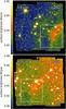 |
Fig. A.1
Entire IRAC images containing the core L260 in the white frame (see also Fig. 2) for 3.6 μm (top) and 4.5 μm (bottom), respectively. |
| Open with DEXTER | |
In former work, constant Ioff were determined by circular averages around the core (e.g., Nielbock et al. 2012) or choosing the local region near the core with the lowest surface brightness (e.g., Stutz et al. 2009). For cuts through the image, variations have also been used, e.g., by linearly interpolating Ioff from locations left and right from the core (e.g., Steinacker et al. 2010; Andersen et al. 2013).
As is visible from the extinction features of cores at 8 μm (see, e.g., Pagani et al. 2010b), almost all cores have a shape deviating from simple spherical symmetry. Judging where outer parts of the core gas are located and where we are looking at variations in the foreground or background gas is therefore difficult, especially for cores near the Galactic plane when the LoS likely crosses other regions.
In the following, we use the core L260 with the strongest coreshine surface brightness in our sample to illustrate how we have performed the off-core measurement and how the results depend on the choice of the background.
In Fig. A.1, the two IRAC images are shown for L260 in the bands 3.6 μm (top) and 4.5 μm (bottom), respectively. The white frame shows the region around the core that is used for the top panels in Fig. 5. As is visible from both images, there is a large scale horizontal gradient across the background of the core.
We have chosen three spots near the core to measure Ioff and indicate their location in panel A of Fig. A.2 as numbered white frames. We also give for comparison the frame 0 in which we measured R. In panel B we show the number distributions of pixels as a function of their surface brightness for the entire IRAC image. The distributions contain the stellar sources that are visible in the high SFB wing of the distribution as they are above the mean SFB of each frame: the frame around Core (A), the off-frames 1-3, and the R-measurement frame 0. The gradients visible in the IRAC image results in a mean surface brightness shift from 1 to 3. We therefore interpolate Ioff from 1 and 3 which leads to a value close to the mean surface brightness seen in frame 2.
The situation changes for 4.5 μm. Using the same frames as indicated in panel C, the surface brightness distributions in frames 2 and 3 are almost identical. Nevertheless, the gradient between 1 and 3 remains, and we also interpolate Ioff at 4.5 μm from both frames.
To estimate the uncertainty in the derived range of observable R, we compare the mean R from interpolating between 1 and 3 and between 2 and 3. Using the mean surface brightnesses of the four frames, we get R = 2.3 for frame 1 to 3 off measurement, and R = 2.41 for frames 2 to 3. We performed this procedure of testing the variation in various frames for all sources discussed here.
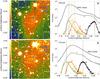 |
Fig. A.2
Background choice for L260. |
| Open with DEXTER | |
Appendix B: Mie calculations
The absorption and scattering coefficients of large grains can be exactly computed for spherical particules only using Mie theory (Bohren & Huffman 1983). Other grain shapes rely on approximate numerical models, or their validity is restricted to small grain sizes.
In this study the water optical constants are extracted from the database of Hudgins et al. (1993). The silicate data are taken from Draine & Lee (1984), and the amorphous carbon data are provided by Zubko et al. (1996).
To simulate porous grains, we use an effective medium formulation where the inclusions are made of vacuum. Amorphous carbon is also considered as inclusions in the silicate matrix.
Consider a particulate composite consisting of a matrix and including various sizes and shapes made of material other than the matrix. Under certain conditions, the composite can be homogenized; i.e., the composite can be replaced by a homogeneous dielectric medium with the same macroscopic electromagnetic response and a certain effective permittivity. Landau & Lifshitz (1960) and independently Looyenga (1965) proposed an effective medium formulation that take inclusion connections for all volume fractionss into account (hereafter LLL model). The effective dielectic function is a volume-fraction weighted-average of the spherical constituents for the composite and is correct to the second order in the differences in permittivities, although dipole-dipole interaction is still not taken into account. For N constituents, the effective dielectric function is  (B.1)
(B.1)
where ϵi is the dielectric function of the material i, and fi are the volume fractions of arbitrary shape. Here, N is the total number of inclusions of a given composition. The sum of all volume fractions has to be lower than 1. For two constituents, the formulation is extremely simple: ![]() (B.2)where ϵmat is the dielectric function of the matrix. It is clear that the LLL model is symmetric with respect to the constituents. Other formulations of the effective medium dielectric function exist (Maxwell Garnett 1904; Bruggeman 1935), each of them with their own strengths and weaknesses. We chose to use the LLL model for its validity for all volume fractions.
(B.2)where ϵmat is the dielectric function of the matrix. It is clear that the LLL model is symmetric with respect to the constituents. Other formulations of the effective medium dielectric function exist (Maxwell Garnett 1904; Bruggeman 1935), each of them with their own strengths and weaknesses. We chose to use the LLL model for its validity for all volume fractions.
Water ice is assumed to form a mantle on the top of the porous silicate + amorphous carbon core. Absorption and scattering cross-sections, as well as the phase-functions for ice-coated porous spherical grains, are computed using the latest version of the Mie routine for coated spheres provided by Toon & Ackerman (1981).
© ESO, 2015
Current usage metrics show cumulative count of Article Views (full-text article views including HTML views, PDF and ePub downloads, according to the available data) and Abstracts Views on Vision4Press platform.
Data correspond to usage on the plateform after 2015. The current usage metrics is available 48-96 hours after online publication and is updated daily on week days.
Initial download of the metrics may take a while.