| Issue |
A&A
Volume 578, June 2015
|
|
|---|---|---|
| Article Number | A10 | |
| Number of page(s) | 12 | |
| Section | Cosmology (including clusters of galaxies) | |
| DOI | https://doi.org/10.1051/0004-6361/201424456 | |
| Published online | 22 May 2015 | |
Online material
Appendix A: CosmicPy package
|
Listing 1
Example of 3D SFB and tomographic Fisher matrix computations using CosmicPy. |
|
| Open with DEXTER | |
CosmicPy is an interactive Python package that allows for simple cosmological computations. Designed to be modular, well-documented and easily extensible, this package aims to be a convenient tool for forecasting cosmological parameter constraints for different probes and different statistics. Currently, the package includes basic functionalities such as cosmological distances and matter power spectra (based on Eisenstein & Hu 1998; and Smith et al. 2003), and facilities for computing tomographic (using the Limber approximation) and 3D SFB power spectra for galaxy clustering and the associated Fisher matrices.
Listing 1 illustrates how CosmicPy can be used to easily compute the 3D SFB Fisher matrix, extract the figure of merit, and generate the associated corner plot similar to Fig. 3.
The full documentation of the package and a number of tutorials demonstrating how to use the different functionalities and reproduce the results of this paper is provided at the CosmicPy webpage: http://cosmicpy.github.io
Although CosmicPy is primarily written in Python for code readability, it also includes a simple interface to C/C++, allowing critical parts of the codes to have a fast C++ implementation as well as enabling existing codes to be easily interfaced with CosmicPy.
Contributions to the package are very welcome and can be in the form of feedback, requests for additional features, documentation, or even code contributions. This is made simple through the GitHub hosting of the project at https://github.com/cosmicpy/cosmicpy
Appendix B: Computing the SFB covariance matrix
Performing a Fisher analysis requires computing the SFB covariance matrix, and more importantly, computing the inverse of this matrix. This last step can be quite challenging as the covariance of the spherical Fourier-Bessel coefficients is a continuous quantity Cℓ(k,k′). Two approaches can be considered to define a covariance matrix in this situation: (i) only using the diagonal covariance Cℓ(ki,ki) at discrete points ki (advocated by Nicola et al. 2014); or (ii) binning Cℓ(k,k′) into bins of size Δk. However, by neglecting the correlation between neighbouring wavenumbers, the first approach overestimates the information content if the interval between wavenumbers is too small, while the second approach would lose information for bins of increasing size and become numerically challenging to invert for bins too small. Another problem is to select the largest scale kmin to include in the covariance matrix. Indeed, Cℓ(k,k) becomes extremely small and numerically challenging to compute for very small k, but small wavenumbers can still potentially contribute to the Fisher information. A careful study is necessary to select a kmin that does not lose information.
Instead, using the kln sampling defined by Eq. (23)naturally introduces a minimum wavenumber and a discrete sampling of scales that preserves all the information. As an added benefit, this approach yields numerically invertible covariance matrices in practice for sensible choices of the boundary condition rmax. Indeed, as ![]() , the choice of cut-off radius sets the fineness of the Cℓ(n,n′) matrix and affects its condition number. However, we find that the Fisher information remains largely unaffected by varying rmax above a certain distance because cutting the very end of the galaxy distribution has little effect. In practice, we have arbitrarily set rmax to the comoving distance at which φ(r) reaches 10-5 of its maximum value. This choice has proven stable in all situations considered in this work. The robustness of our computation of the Fisher matrix with respect to the choice of rmax is illustrated in Fig. B.1, where we show the contributions of each angular mode to the Fisher matrix element
, the choice of cut-off radius sets the fineness of the Cℓ(n,n′) matrix and affects its condition number. However, we find that the Fisher information remains largely unaffected by varying rmax above a certain distance because cutting the very end of the galaxy distribution has little effect. In practice, we have arbitrarily set rmax to the comoving distance at which φ(r) reaches 10-5 of its maximum value. This choice has proven stable in all situations considered in this work. The robustness of our computation of the Fisher matrix with respect to the choice of rmax is illustrated in Fig. B.1, where we show the contributions of each angular mode to the Fisher matrix element ![]() . Our empirical choice for rmax in this case is 5420 h-1 Mpc, but the results are not affected by increasing rmax to 5700 h-1 Mpc even more.
. Our empirical choice for rmax in this case is 5420 h-1 Mpc, but the results are not affected by increasing rmax to 5700 h-1 Mpc even more.
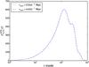 |
Fig. B.1
Contribution to the SFB Fisher matrix element |
| Open with DEXTER | |
Appendix C: Deriving the spherical Fourier-Bessel shot noise power spectrum
Here, we derive the expression of the shot noise by discretising the survey in cells that either contain one or zero galaxies (Peebles 1980). This method was used in Heavens et al. (2006) to yield the expression of the shot noise in the case of 3D cosmic shear. We considered a point process defined on small cells c, each of which contains nc = 0 or 1 depending on whether the cell contains a galaxy or not:  (C.1)where δc(r) = 1 if r is within the cell c, 0 otherwise, and where nc fulfils (Peebles 1980)
 ![]() (C.2)where Δc is the volume of cell c and
(C.2)where Δc is the volume of cell c and ![]() is the average number density of galaxies of the survey at distance rc. Furthermore, the cross-term for c ≠ d is
is the average number density of galaxies of the survey at distance rc. Furthermore, the cross-term for c ≠ d is ![]() (C.3)The SFB expansion of the density field can now be expressed as a sum over small cells c:
(C.3)The SFB expansion of the density field can now be expressed as a sum over small cells c:  (C.4)\newpage\noindentFrom this expression, we can derive the two-point correlation function of this field:
 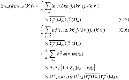 In the last equation, the first term for c = d contains the shot noise contribution and the second term contains the monopole contribution and the correlation function of the density fluctuations. Returning to continuous integration by decreasing the volume of cells Δc, we have
 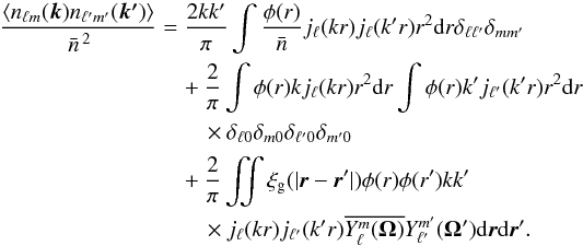 (C.7)Therefore, in this expression, we recognize three terms:
-
the shot noise contribution, onlyfor l = l′ and m = m′:
 (C.8)
(C.8) -
the contribution from the power spectrum, only for l = l′ and m = m′:
 (C.10)
 (C.11)
© ESO, 2015
Current usage metrics show cumulative count of Article Views (full-text article views including HTML views, PDF and ePub downloads, according to the available data) and Abstracts Views on Vision4Press platform.
Data correspond to usage on the plateform after 2015. The current usage metrics is available 48-96 hours after online publication and is updated daily on week days.
Initial download of the metrics may take a while.