| Issue |
A&A
Volume 576, April 2015
|
|
|---|---|---|
| Article Number | A4 | |
| Number of page(s) | 12 | |
| Section | The Sun | |
| DOI | https://doi.org/10.1051/0004-6361/201424646 | |
| Published online | 13 March 2015 | |
Online material
Appendix A: Reconnection rate
When the general theory of reconnection was developed, an elegant derivation of the reconnection rate was presented that makes use of an Euler potential representation of the magnetic field (Hesse & Schindler 1988; Schindler 2007). Here we present an alternative derivation, based on Cartesian tensors, for resistive MHD. Consider magnetic field lines passing through a non-ideal region ![]() . Inside this region, the resistivity η ≠ 0. Outside is an ideal plasma, where η = 0. Consider a closed path that passes though
. Inside this region, the resistivity η ≠ 0. Outside is an ideal plasma, where η = 0. Consider a closed path that passes though ![]() parallel to a magnetic field line, as shown in Fig. A.1.
parallel to a magnetic field line, as shown in Fig. A.1.
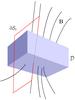 |
Fig. A.1
Magnetic field lines passing through a non-ideal region |
| Open with DEXTER | |
Let ![]() denote the surface bounded by the closed path. The rate of reconnection is the rate of change of flux Φ through the surface
denote the surface bounded by the closed path. The rate of reconnection is the rate of change of flux Φ through the surface 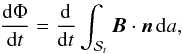 where n is the unit normal to the surface
 ![]() . In order to differentiate the integral with respect to time, one must move from an Eulerian frame to a Lagrangian one. This can be achieved via an application of Nanson’s formula to give
. In order to differentiate the integral with respect to time, one must move from an Eulerian frame to a Lagrangian one. This can be achieved via an application of Nanson’s formula to give 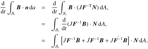 Here, geometric quantities that are now written in captials are relative to a Lagrangian frame with surface
 ![]() , e.g. n is Eulerian and N is Lagrangian. F = ∂x/∂X is the deformation gradient, a second order Cartesian tensor relating the Lagrangian and Eulerian frames. Associated with this is J = det(F). In the last integral, dots over terms represent differentiation with respect to time. It can be shown that
, e.g. n is Eulerian and N is Lagrangian. F = ∂x/∂X is the deformation gradient, a second order Cartesian tensor relating the Lagrangian and Eulerian frames. Associated with this is J = det(F). In the last integral, dots over terms represent differentiation with respect to time. It can be shown that ![]() where L = ∂u/∂x. Here, u is the Eulerian velocity, making L an entirely Eulerian tensor. It can also be shown that
where L = ∂u/∂x. Here, u is the Eulerian velocity, making L an entirely Eulerian tensor. It can also be shown that ![]() by differentiating the expression FF-1 = I. Collecting these results together, it follows that
by differentiating the expression FF-1 = I. Collecting these results together, it follows that 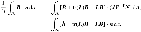 By expressing the integrand in terms of vectors and making use of the resistive induction equation, one finds
 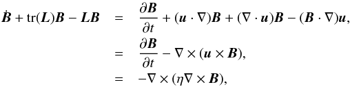 where η = η(x) is the resistivity. By an application of Stokes’ theorem, one can show that
 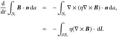 Taking the dot product of a unit vector
 ![]() with the resistive Ohm’s law gives
with the resistive Ohm’s law gives ![]() where η = (μ0σ)-1 with conductivity σ = σ(x) and (constant) magnetic permeability μ0. As η = 0 outside
where η = (μ0σ)-1 with conductivity σ = σ(x) and (constant) magnetic permeability μ0. As η = 0 outside ![]() , the integration only gives a non-zero value along the section of the path inside
, the integration only gives a non-zero value along the section of the path inside ![]() (the green path in Fig. A.1). If this section is labelled Γ, it follows that
(the green path in Fig. A.1). If this section is labelled Γ, it follows that 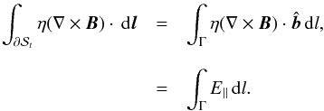 It then follows that
 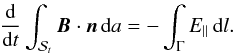 The choice of field line, and hence path, taken through
 ![]() was arbitrary. Therefore, it is common to choose the field line that returns the largest magnitude. Since, in this work, we are integrating along field lines that pass through points connecting all four flux systems (four-colour points), the reconnection rate ℛ(t) is taken to be
was arbitrary. Therefore, it is common to choose the field line that returns the largest magnitude. Since, in this work, we are integrating along field lines that pass through points connecting all four flux systems (four-colour points), the reconnection rate ℛ(t) is taken to be 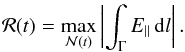 Here the integration is along the field line that gives the largest magnitude for the integrated parallel electric field.
 ![]() is the set of field lines that pass through four-colour points, and varies in time. Γ is the path along the field line in the current sheet.
is the set of field lines that pass through four-colour points, and varies in time. Γ is the path along the field line in the current sheet.
© ESO, 2015
Current usage metrics show cumulative count of Article Views (full-text article views including HTML views, PDF and ePub downloads, according to the available data) and Abstracts Views on Vision4Press platform.
Data correspond to usage on the plateform after 2015. The current usage metrics is available 48-96 hours after online publication and is updated daily on week days.
Initial download of the metrics may take a while.