| Issue |
A&A
Volume 576, April 2015
|
|
|---|---|---|
| Article Number | A104 | |
| Number of page(s) | 33 | |
| Section | Interstellar and circumstellar matter | |
| DOI | https://doi.org/10.1051/0004-6361/201424082 | |
| Published online | 13 April 2015 | |
Online material
Appendix A: Noise estimates for Planck smoothed maps
Here, we show how to smooth polarization maps and derive the covariance matrix associated to the smoothed maps.
Appendix A.1: Analytical expressions for smoothing maps of the Stokes parameters and noise covariance matrices
Smoothing total intensity maps is straightforward, but this is not the case for polarization maps. Because the polarization frame follows the sky coordinates and rotates from one centre pixel to a neighbouring pixel whose polarization will be included in the smoothing, in principle the (Q,U) doublet must be also rotated at the same time (e.g., Keegstra et al. 1997). The issue is similar for evaluating the effects of smoothing on the 3 × 3 noise covariance matrix, though with mathematically distinct results. In this Appendix, we present an exact analytical solution to the local smoothing of maps of the Stokes I, Q, and U, as well as the effects of smoothing on their corresponding noise covariance matrix.
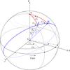 |
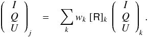
Fig. A.1
Definition of points and angles on the sphere involved in the geometry of the smoothing of polarization maps (adapted from Keegstra et al. 1997). J is the position of the centre of the smoothing beam, and K a neighbouring pixel, with spherical coordinates (ϕ⋆, θ⋆) and (ϕk, θk), respectively. The great circle passing through J and K is shown in blue. The position angles ψ⋆ and ψk here are in the HEALPix convention, increasing from Galactic north toward decreasing Galactic longitude (west) on the celestial sphere as seen by the observer at O. |
| Open with DEXTER | |
Appendix A.1.1: Smoothing of Stokes parameters
Figure A.1 presents the geometry of the
problem. Let us consider a HEALPix pixel j at point
J on the celestial
sphere, with spherical coordinates (ϕ⋆,θ⋆). To perform
smoothing around this position with a Gaussian beam with standard deviation
σ1 / 2 =
FWHM/ 2.35 centred at the position of this
pixel we select all HEALPix pixels that fall within 5 times
the FWHM of the smoothing beam (this footprint is sufficient for all practical
purposes). Let k be one such pixel, centred at the point
K with coordinates
(ϕk,
θk), at angular
distance β from J defined by ![]() (A.1)The normalized Gaussian weight is then
(A.1)The normalized Gaussian weight is then
 (A.2)and ∑
kwk =
1. Before averaging in the Gaussian beam, we need to rotate the
polarization reference frame in K so as align it with that in J. For that the reference frame is
first rotated by ψk into the
great circle running through K and J, then translated to J, and finally rotated through −ψ⋆. The net
rotation angle of the reference frame from point K to point J is then
(A.2)and ∑
kwk =
1. Before averaging in the Gaussian beam, we need to rotate the
polarization reference frame in K so as align it with that in J. For that the reference frame is
first rotated by ψk into the
great circle running through K and J, then translated to J, and finally rotated through −ψ⋆. The net
rotation angle of the reference frame from point K to point J is then ![]() (A.3)Due to the cylindrical symmetry around
axis z,
evaluating
(A.3)Due to the cylindrical symmetry around
axis z,
evaluating ![]() does not depend on the longitudes
ϕ⋆ and
ϕk taken
separately, but only on their difference
does not depend on the longitudes
ϕ⋆ and
ϕk taken
separately, but only on their difference
![]() (A.4)Using spherical trigonometry in Fig.
A.1 with the HEALPix
convention for angles ψ⋆ and
ψk, we find:
(A.4)Using spherical trigonometry in Fig.
A.1 with the HEALPix
convention for angles ψ⋆ and
ψk, we find:
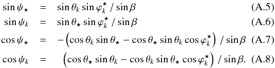 To derive ψk and
ψ⋆ we use the
two-parameter arctan
function that resolves the π ambiguity in angles:
To derive ψk and
ψ⋆ we use the
two-parameter arctan
function that resolves the π ambiguity in angles: ![]() (A.9)Because of the tan implicitly used, sinβ (a positive
quantity) is eliminated in the evaluation of ψ⋆, ψk, and
(A.9)Because of the tan implicitly used, sinβ (a positive
quantity) is eliminated in the evaluation of ψ⋆, ψk, and
![]() .
.
We can now proceed to the rotation. It is equivalent to rotate the polarization
frame at point K by the
angle ![]() , or to rotate the data triplet
(Ik, Qk, Uk) at point
K by an angle
, or to rotate the data triplet
(Ik, Qk, Uk) at point
K by an angle
![]() around the axis I. The latter is done
with the rotation matrix (e.g., Tegmark & de
Oliveira-Costa 2001)
around the axis I. The latter is done
with the rotation matrix (e.g., Tegmark & de
Oliveira-Costa 2001) 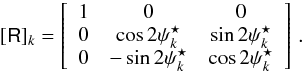 (A.10)Finally, the smoothed I, Q, and U maps are calculated by:
 (A.11)
Appendix A.1.2: Computing the noise covariance matrix for smoothed polarization maps
We want to compute the noise covariance matrix [ C] ⋆ at
the position of a HEALPix pixel j for the smoothed
polarization maps, given the noise covariance matrix [ C ] at the higher resolution of the
original data. We will assume that the noise in different pixels is uncorrelated.
From the given covariance matrix [ C ]
k at any pixel k we can produce
random realizations of Gaussian noise through the Cholesky decomposition of the
covariance matrix: 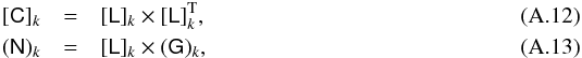 where in the decomposition
![]() is the transpose of the matrix
[ L ]
k and (G)k =
(GI,GQ,GU)k
is a vector of normal Gaussian variables for I, Q, and
U.
is the transpose of the matrix
[ L ]
k and (G)k =
(GI,GQ,GU)k
is a vector of normal Gaussian variables for I, Q, and
U.
Applying Eq. (A.11) to the Gaussian
noise realization, we obtain
 (A.14)The covariance matrix of the smoothed
at the position J is
given by
(A.14)The covariance matrix of the smoothed
at the position J is
given by 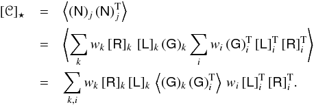 (A.15)If the noise in distinct pixels is
independent, as assumed, then ⟨
(G)k (G)i ⟩ =
δki, the Kronecker
symbol, and so
(A.15)If the noise in distinct pixels is
independent, as assumed, then ⟨
(G)k (G)i ⟩ =
δki, the Kronecker
symbol, and so  (A.16)which can be computed easily with Eq.
(A.10).
(A.16)which can be computed easily with Eq.
(A.10).
Developing each term of the matrix, we can see more explicitly how the smoothing
mixes the different elements9 of the noise
covariance matrix:  where we note that
![]() and
and
![]() depend on j and k. The mixing of the
different elements of the covariance matrix during the smoothing is due not to the
smoothing itself, but to the rotation of the polarization frame within the smoothing
beam.
depend on j and k. The mixing of the
different elements of the covariance matrix during the smoothing is due not to the
smoothing itself, but to the rotation of the polarization frame within the smoothing
beam.
Appendix A.1.3: Smoothing of the noise covariance matrix with a Monte Carlo approach
For the purpose of this paper, we obtained smoothed covariance matrices using a Monte Carlo approach.
We first generate correlated noise maps (nl, nQ,
nU) on I, Q, and U at the resolution of the data using
 (A.23)where Gl,
GQ, and GU are
Gaussian normalized random vectors and L is the Cholesky decomposition of the
covariance matrix [ C ]
defined in Eq. (A.12).
(A.23)where Gl,
GQ, and GU are
Gaussian normalized random vectors and L is the Cholesky decomposition of the
covariance matrix [ C ]
defined in Eq. (A.12).
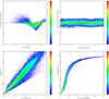 |
Fig. B.1
Upper panels: difference between the conventional and the Bayesian mean posterior estimates of p and ψ as a function of the conventional estimate. Lower panels: Bayesian mean posterior estimates of σp and σψ as a function of the conventional estimate. The dashed red lines show where the two methods give the same result. Each plot shows the density of points in log-scale for the Planck data at 1° resolution. The dotted line in the lower right plot shows the value for pure noise. The colour scale shows the pixel density on a log10 scale. |
| Open with DEXTER | |
The above noise I, Q, an U maps are then smoothed to the requested resolution using the smoothing procedure of the HEALPix package. The noise maps are further resampled using the udgrade procedure of the HEALPix package, so that pixellization respects the Shannon theorem for the desired resolution. The smoothed covariance matrices for each sky pixel are then derived from the statistics of the smoothed noise maps. The Monte Carlo simulations have been performed using 1000 realizations.
Both the analytical and the Monte Carlo approaches have been estimated on the Planck data and shown to give equivalent results.
Appendix B: Debiasing methods
Because p is a quadratic function of the observed Stokes parameters (see Eq. (1)) it is affected by a positive bias in the presence of noise. The bias becomes dominant at low S/N. Below we describe briefly a few of the techniques that have been investigated in order to correct for this bias. For a full discussion of the various debiasing methods, see the introductions in Montier et al. (2015a,b) and references therein.
Appendix B.1: Conventional method (method 1)
This method is the conventional determination often used on extinction polarization data. It uses the internal variances provided with the Planck data, which includes the white noise estimate on the total intensity (CII) as well as on the Q and U Stokes parameters (CQQ and CUU) and the off-diagonal terms of the noise covariance matrix (CIQ,CIU,CQU).
The debiased p2 values are computed using
![]() (B.1)where
(B.1)where
![]() is the variance of p computed from the
observed Stokes parameters and the associated variances as follows:
is the variance of p computed from the
observed Stokes parameters and the associated variances as follows: 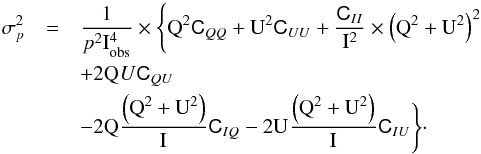 (B.2)The uncertainty on ψ is given by
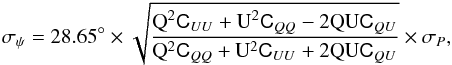 (B.3)where σP is the uncertainty
on the polarized intensity:
(B.3)where σP is the uncertainty
on the polarized intensity: ![]() (B.4)In the case where I is supposed to be
perfectly known, CII = CIQ =
CIU = 0,
(B.4)In the case where I is supposed to be
perfectly known, CII = CIQ =
CIU = 0, 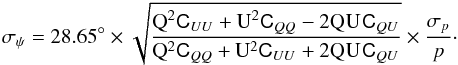 (B.5)Because it is based on derivatives around
the true value of the I,
Q, and U parameters, this is only valid in the
high S/N regime. The conventional values of uncertainties derived above are compared
to the ones obtained using the Bayesian approach in Fig. B.1.
(B.5)Because it is based on derivatives around
the true value of the I,
Q, and U parameters, this is only valid in the
high S/N regime. The conventional values of uncertainties derived above are compared
to the ones obtained using the Bayesian approach in Fig. B.1.
Appendix B.2: Time cross-product method (method 2)
This method consists in computing cross products between estimates of Q and U with independent noise properties. In the case of Planck HFI, each sky pixel has been observed at least four times and the four independent surveys can be used for this purpose. Another option is to use half-ring maps which have been produced from the first and second halves of each ring. These methods have the disadvantage of using only part of the data, but the advantage of efficiently debiasing the data if the noise is effectively independent, without assumptions about the Q and U uncertainties.
In that case, ![]() can be computed as
can be computed as 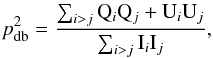 (B.6)where the sum is carried out either over
independent survey maps or half-ring maps.
(B.6)where the sum is carried out either over
independent survey maps or half-ring maps.
The uncertainty of p2 can in turn be evaluated from the
dispersion between pairs  (B.7)
(B.7)
Appendix B.3: Bayesian methods (method3)
We use a method based on the one proposed by Quinn (2012) and extended to the more general case of an arbitrary covariance matrix by Montier et al. (2015a). We use the Mean Posterior Bayesian (MB) estimator described in Montier et al. (2015b). Unlike the conventional method presented in Sect. B.1, this method is in principle accurate at any signal-to-noise ratio. Figure B.1 compares the Bayesian predictions for p and ψ and their uncertainties σp and σψ with those obtained from the conventional method (Eqs. (1), (2), and (B.1)–(B.4)) as predicted from the Planck data at 1deg resolution. As can be seen in the figure, the bias on p is generally important even at this low resolution. The conventional uncertainties are accurate only at low uncertainties, as expected because Eqs. (B.4) and (B.5) are obtained from Taylor expansion around the true values of the parameters. The difference in the uncertainties is the greatest for σψ as the true value can only reach 52deg for purely random orientations.
Appendix C: Tests on the bias of 
We have performed tests in which we used the Planck noise covariance
matrices in order to check that the structures we observe in the maps of the
polarization angle dispersion function ![]() are not caused by systematic noise bias. One of the tests (called
are not caused by systematic noise bias. One of the tests (called
![]() ) consisted of assigning each
pixel a random polarization angle ψ. The second one (called
) consisted of assigning each
pixel a random polarization angle ψ. The second one (called
![]() ) consisted of setting
ψ to a
constant value over the whole sky map, which leads to
) consisted of setting
ψ to a
constant value over the whole sky map, which leads to
![]() (except near the poles). In that
case, changing ψ in the data was done while preserving the value
of p and
σp computed as in Eq.
(B.2), through the appropriate
modification of I,
Q, and U. The tests also use the noise covariance
of the data, so that the tests are performed with the same sky distribution of the
polarization S/N as in the data. This is critical for investigating the spatial
distribution of the noise-induced bias on
(except near the poles). In that
case, changing ψ in the data was done while preserving the value
of p and
σp computed as in Eq.
(B.2), through the appropriate
modification of I,
Q, and U. The tests also use the noise covariance
of the data, so that the tests are performed with the same sky distribution of the
polarization S/N as in the data. This is critical for investigating the spatial
distribution of the noise-induced bias on ![]() .
In both tests, we added correlated noise on I, Q,
and U using the actual noise
covariance matrix at each pixel, and computed the map of
.
In both tests, we added correlated noise on I, Q,
and U using the actual noise
covariance matrix at each pixel, and computed the map of
![]() using Eq. (6) and the same lag value as
for the Planck data.
using Eq. (6) and the same lag value as
for the Planck data.
Figure C.1 (upper) shows the histograms of the
![]() values obtained for these two tests, both for the whole sky and in the mask used in the
analysis of the real data. histograms peak at the value of
values obtained for these two tests, both for the whole sky and in the mask used in the
analysis of the real data. histograms peak at the value of
![]() for Gaussian noise only (no signal,
for Gaussian noise only (no signal, ![]() ). The corresponding map of
). The corresponding map of
![]() does not exhibit the filamentary structure of the actual data shown in Fig. 12. Similarly, the test histograms of
does not exhibit the filamentary structure of the actual data shown in Fig. 12. Similarly, the test histograms of
![]() do not resemble that of the real data shown in Fig. 14.
do not resemble that of the real data shown in Fig. 14.
The ![]() test is important for assessing
the amplitude of the noise-induced bias, as Monte Carlo simulations show that assuming a
true value of
test is important for assessing
the amplitude of the noise-induced bias, as Monte Carlo simulations show that assuming a
true value of ![]() maximizes the bias. We therefore
use this test as a determination of the upper limit for the bias given the polarization
fraction and noise properties of the data. Figure C.1 (upper) shows that the histograms of the recovered values peak at
maximizes the bias. We therefore
use this test as a determination of the upper limit for the bias given the polarization
fraction and noise properties of the data. Figure C.1 (upper) shows that the histograms of the recovered values peak at
![]() . The histogram is also narrower
in the high
. The histogram is also narrower
in the high ![]() S/N region than over larger sky regions at lower S/N. In the high
S/N region than over larger sky regions at lower S/N. In the high
![]() S/N mask, 60% of the data
points have a noise-induced bias smaller than 1.6°, and 97% have a bias smaller than 9.6°. The maps of the bias computed for
this test show a correlation with the map of
S/N mask, 60% of the data
points have a noise-induced bias smaller than 1.6°, and 97% have a bias smaller than 9.6°. The maps of the bias computed for
this test show a correlation with the map of ![]() .
However, as shown in Fig. C.1 (lower panel), the
effect of the bias (the size of the offset) is small at high values of
.
However, as shown in Fig. C.1 (lower panel), the
effect of the bias (the size of the offset) is small at high values of
![]() for most pixels and can reach up to 50% for a larger fraction of points at lower
for most pixels and can reach up to 50% for a larger fraction of points at lower
![]() values (say below
values (say below ![]() ). This
). This
bias correction does not significantly change the structure of the map shown in Fig.
12 and so, in particular, bias does not cause
the filamentary structures observed. We note, however, that the noise-induced bias can
change the slope of the correlation between ![]() and p.
and p.
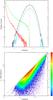 |
Fig. C.1
Upper: histogram of |
| Open with DEXTER | |
© ESO, 2015
Current usage metrics show cumulative count of Article Views (full-text article views including HTML views, PDF and ePub downloads, according to the available data) and Abstracts Views on Vision4Press platform.
Data correspond to usage on the plateform after 2015. The current usage metrics is available 48-96 hours after online publication and is updated daily on week days.
Initial download of the metrics may take a while.