| Issue |
A&A
Volume 575, March 2015
|
|
|---|---|---|
| Article Number | A55 | |
| Number of page(s) | 22 | |
| Section | Extragalactic astronomy | |
| DOI | https://doi.org/10.1051/0004-6361/201425081 | |
| Published online | 23 February 2015 | |
Online material
Appendix A: Flare decomposition method
The detection and parametrisation of different flares (which are then used to compute the associated variability brightness temperature) requires solving several problems, most of which have to do with the paradox that before an independent parameterisation of all flares is reached, we need to identify their average shape and spectral evolution, minimise the arbitrariness of the results. The problems to be addressed can be summarised as follows:
-
1.
We need to identify of the strongest flare, accounting for the fact that its amplitude may strongly depend on frequency so that the strongest flare at one frequency may be a minor event at others.
-
2.
We also need to localise of the same flare at different frequencies, given its spectral evolution.
-
3.
The flares need to be modelled efficiently using the minimum number of free parameters.
-
4.
Finally, we have to test and possibly correct the model to optimise the results.
The implementation of these steps was made as follows:
-
1.
We estimated the average time delays between the flux density variations detected in different light curves. The main complication in this procedure is the fact that using a standard cross-correlation function (see Edelson & Krolik 1988; Lehar et al. 1992) on pairs of light curves does not ensure consistent results. For example, assuming the estimated delays between three light curves a, b, and c to be τa,b, τa,c and τb,c, it might well be that τa,c ≠ τa,b + τb,c. A solution of this problem is to include all the possible pairs of light curves when calculating the time delays. By visual inspection, a maximum time delay between light curves, τmax, is identified. Then, for every pair of light curves i and j with i<j, a cross-correlation function ri,j(τi,j) is calculated for any time delay τi,j in the range (−τmax,τmax). For n monitored frequencies an overall correlation function can be calculated as
 (A.1)where
 We
computed R for any possible set of time delays,
excluding all the combinations involving ri,j(τi,j)
< 0. The most significant set of time
delays was selected as the one providing the highest overall correlation value.
We
computed R for any possible set of time delays,
excluding all the combinations involving ri,j(τi,j)
< 0. The most significant set of time
delays was selected as the one providing the highest overall correlation value.
-
2.
We composed a “cumulative” light curve, in which the strongest flare was identified. The light curves were shifted in time by the best fit delays found in the previous step, so that their variations were aligned. Their fluxes were normalised by their standard deviation, to have similar variations at all wavelengths. Assuming for example that all the variations at 86.24 GHz have an amplitude of 1 Jy and at 2.64 GHz have an amplitude of 0. Jy, they all count the same for the identification of the flares. This way, we ensured that our detection algorithm was not biased towards the highest frequencies. The resulting light curves were merged to create one well-sampled total “cumulative” light curve. The merging of the light curves does not require averaging; the points from all the light curves are combined regardless of the frequency at which they were observed. The previous steps are meant to make all points equivalent, giving us the opportunity create a well-sampled light curve in which every data point from every frequency participates with the same weight. To construct the cumulative light curve, one could identify the following steps:
-
3.
We identified the strongest flare. The cumulative light curve was smoothed (with an adaptive smoothing factor) and localised the highest flux density.
-
4.
We localised the same flare at different frequencies. Knowing the average time delays between variations occurring at different frequencies, the strongest flare can be identified in each of the actual light curves. Gaussian fit models, different for each wavelength, were applied to the actual light curves to determine the amplitude and timescale of the strongest flare; they were then subtracted from the original flux densities, creating a new set of light curves (one per wavelength) for which all the steps from step 3 on are repeated. The procedure was iterated until no other significant flares are detected.
-
5.
Model test. The residual light curves were checked to verify that no peaks or dips are systematically present in the position of the subtracted flares. Their existence would indicate that the flares are not properly modelled; new models would be created and the whole procedure repeated until a satisfactory result is reached.
This approach has the advantage of individually localising and modelling each event. Once a flare is detected in a cumulative light curve, the average time delays returned by step 1 allow us to infer its approximate position in the real light curves. The accurate position is then identified from the flux peak closest to the approximate position. In this way, we are able to estimate the actual time delays as a function of wavelength for each flare separately, and therefore detect possible variations in their spectral evolution. Naturally, the procedure also provides information about how the amplitude and the rising and decaying times of the flares vary with wavelength, which leads to a full parametrisation of the flux density variations observed in the sources; this is necessary to compute brightness temperatures.
Appendix B: Results of the flare decomposition
Here we append the results of the flare decomposition method described in Sect. 5.1.
Results of the flare decomposition for all three sources.
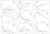 |
Fig. B.1
Left column: J0324+3410: top panel: amplitude of the detected flares as a function of observing frequency with the cycle labels corresponding to the events seen in Fig. 2; middle panel: flare delays; bottom panel: Tvar for the different activity cycles (flares) as a function of observing frequency. Middle column: J0948+0022. Right column: J1505+0326. |
| Open with DEXTER | |
© ESO, 2015
Current usage metrics show cumulative count of Article Views (full-text article views including HTML views, PDF and ePub downloads, according to the available data) and Abstracts Views on Vision4Press platform.
Data correspond to usage on the plateform after 2015. The current usage metrics is available 48-96 hours after online publication and is updated daily on week days.
Initial download of the metrics may take a while.