| Issue |
A&A
Volume 570, October 2014
|
|
|---|---|---|
| Article Number | A124 | |
| Number of page(s) | 23 | |
| Section | The Sun | |
| DOI | https://doi.org/10.1051/0004-6361/201424124 | |
| Published online | 03 November 2014 | |
Online material
Appendix A: Collision strength approximations and their accuracy
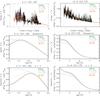 |
Fig. A.1
Examples of the collision strengths. Top: original collision strengths Ωij(Ei) (black) for the 1404.16 Å transition in O iv (left) and the 257.77 Å transition in Fe xi (right). The colored lines correspond to the four averaging methods (Appendix A). Middle: Maxwellian Υji for these transitions together with the Υs obtained using the averaged ⟨ Ωij(Ei) ⟩. Bottom: the same as the middle panel for κ = 2. |
| Open with DEXTER | |
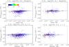 |
Fig. A.2
Relative error of the distribution-averaged collision strengths for O iv and Fe xi, produced using Method 4 (Appendix A), is shown for two extreme cases: Maxwellian distribution (top) and κ = 2 (bottom). The temperature corresponds to the maximum of the relative ion abundance. |
| Open with DEXTER | |
Because of the large number of transitions in the Fe ions, the Ωji datafiles are several tens of GiB large. This hampers effective storage, handling, and publishing of such large datasets. Furthermore, calculations for some ions do not contain  points, but up to one order of magnitude more. An example is the O iv calculations done by Liang et al. (2012), which contain ≈ 1.87 × 10⁵ points. We note that this ion was partially investigated already by Dudík et al. (2014).
In an effort to overcome the problems posed by the large data volume of the collison strength calculations, we tested whether coarser  grids could be sufficient. To do so, we devised and tested several simple methods of averaging over the Ei points:
-
1.
Averaging over uniformly spaced grid of
points, with  Ryd
Ryd -
2.
Averaging over uniformly spaced grid of
points, with  Ryd
Ryd -
3.
Averaging over uniformly spaced grid in log
 , with Δlog(
-
4.
Averaging over uniformly spaced grid in log
, with Δlog( .
.
An example of the ⟨ Ωji ⟩ obtained by these methods is shown in Fig. A.1 (top row) for O iv and Fe xi. The O iv is used here since its Ωij(Ei) has more than one order of magnitude more energy points than the Fe ix–Fe xiii ions studied in this paper. We note that in Fig. A.1, the
 ji(T,κ) are plotted for κ = 2 instead of Υji(T,κ) because of the exp(ΔEij/kBT) factor present in Eq. (13) reaches very large values for low log(T/K). The level of reduction of points depends strongly on the number of the original points, as well as the original interval covered by the points. Typically, the reduction is about an order of magnitude in case of the less coarse Methods 2 and 4, but can be much larger, e.g. a factor of ≈ 5 × 10³ for O iv and Method 1.
Upon calculation of Υij(T,κ) and
ji(T,κ), we found that Method 1 fails dramatically, since the Υij( ⟨ Ωji ⟩ ΔEi = 1 Ryd) do not match the Υij(Ωji) calculated using the original data. Method 4 gives the best results in terms of most closely matching the Υij(T,κ) and
ji(T,κ) (see Fig. A.1) calculated using original, non-averaged Ωji data. Differences can arise at low log(T/K) because at low log(T/K), the Υij(T,κ) and
ji(T,κ) are dominated by the contribution from the energies near the excitation threshold at Ei = ΔEij. The averaging of Ωji cannot be performed in the energy interval of the coarse Ei grid containing the excitation threshold. As a result, inaccurate extrapolation of the first point of the ⟨ Ωji ⟩ to the energy ΔEij causes departure of the Υij( ⟨ Ωji ⟩ Δlog (Ei/ Ryd) = 0.01) from the Υij(Ωji) calculated using the original Ωji data.
For Method 4, the relative error R, defined as 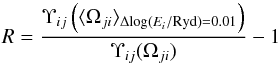 (A.1)is typically only a few per cent (see Fig. A.2). In this figure, we plot the relative error at temperatures corresponding to the temperature of the maximum relative ion abundance (Dzifčáková & Dudík 2013). For the transitions having high rates (i.e. Υij values), the relative error is very small, less than 0.5% (Fig. A.2). The relative error is larger for weaker transitions with lower Υij values. For such transitions, the error is typically a few per cent. However, it can reach ≈20–30% for κ = 2 and weak (unobservable) transitions in O iv.
The O iv and κ = 2 is an extreme case for two reasons. First, the collision strength Ωji for the weak transitions are steeply decreasing with Ei, and thus the values of Υij( ⟨ Ωji ⟩ Δlog (Ei/ Ryd) = 0.01) are dominated by the first energy point. Second, the maximum of the relative ion abundance of the O iv ion is, for κ-distributions, shifted to lower log(T/K) than for the Maxwellian distribution (Dzifčáková & Dudík 2013; Dudík et al. 2014), increasing the error of the calculation. We consider even this value of R = ≈ 20−30% acceptable given the uncertainties in the atomic data calculations, particularly at the excitation threshold. We also note that the strongest transitions have small relative errors of only a few percentage points (Fig. A.2, bottom left).
Appendix B: Selected transitions
A list of the spectral lines selected by the procedure described in Sect. 5.1 are listed in Tables B.1–B.5 together with their selfblends. Wavelengths of the primary (strongest) transition within a selfblend are given together with the energy levels involved. Selfblending transitions are indicated together with their level numbers. Most of the selected spectral lines do not contain any selflblending transitions.
© ESO, 2014
Current usage metrics show cumulative count of Article Views (full-text article views including HTML views, PDF and ePub downloads, according to the available data) and Abstracts Views on Vision4Press platform.
Data correspond to usage on the plateform after 2015. The current usage metrics is available 48-96 hours after online publication and is updated daily on week days.
Initial download of the metrics may take a while.