| Issue |
A&A
Volume 568, August 2014
|
|
|---|---|---|
| Article Number | A22 | |
| Number of page(s) | 32 | |
| Section | Cosmology (including clusters of galaxies) | |
| DOI | https://doi.org/10.1051/0004-6361/201423413 | |
| Published online | 08 August 2014 | |
Online material
Appendix A: Visual inspection
In addition to the software cuts, we performed a visual inspection of the SN light-curve fits. We discarded the following SNe Ia, for which the SALT2 fits were particularly poor20:
-
1.
Fit probability <0.01 due to apparent problems in the photometry: SDSS739⋆, SDSS1316⋆, SDSS3256 (2005hn), SDSS6773 (2005iu), SDSS12780, SDSS12907, SDSS13327⋆, SDSS16287, SDSS16578⋆, SDSS16637⋆, SDSS17176⋆, SDSS18456, SDSS18643, SDSS19381 (2007nk), SDSS20376⋆, SDSS20528 (2007qr), SDSS21810⋆.
-
2.
Poor fit, probable 1986G-like: SDSS17886 (sn2007jh) (Stritzinger et al. 2011).
-
3.
Poor fit, 2002cx-like: SDSS20208 (sn2007qd) (McClelland et al. 2010; Foley et al. 2013).
-
4.
Pathological sampling leading to unstable fit results: SDSS17500⋆, SDSS16692⋆.
We also discarded the following four events that are >3σ outliers on the Hubble diagram:
-
1.
Over-luminous: SDSS14782 (2006jp), SDSS15369 (2006ln).
-
2.
Subluminous: SDSS15459 (2006la), SDSS17568 (2007kb).
Last, a proper and stable determination of the date of maximum is necessary for SNe Ia entering in the training sample, because the date of maximum is held fixed in the training. We looked for remaining poorly sampled light curves in the training sample, and discarded the following nine SNe (only from the training sample):
-
1.
Too few observations after the epoch of peak brightness(despite a reported uncertainty on t0 passing the cuts): SDSS10434, SDSS19899, SDSS20470, SDSS21510.
-
2.
Too few observations before the epoch of peak brightness: SDSS6780, SDSS12781, SDSS12853 (2006ey), SDSS13072, SDSS18768.
Appendix B: Details on calibration systematics
Appendix B.1: Consistency of the CfAIII and CSP photometric calibration
A few low-z SNe Ia have been observed contemporaneously with several telescopes which provides a way to assess their relative calibration. Mosher et al. (2012) studied nine spectroscopically confirmed Type Ia supernova observed by both the CSP and the SDSS-II surveys. The study provides us with stringent constraints on possible differences between the CSP calibration and the SDSS/SNLS calibration of B13. The Mosher et al. (2012) results are reproduced in Table B.1.
Calibration offsets.
Spectroscopically confirmed SNe Ia in common between CSP and CFA.
We performed a similar study on SNe Ia observed by both the CfAIII and CSP surveys. To increase the statistics available for this comparison, we consider SNe Ia from both the first (Contreras et al. 2010) and second (Stritzinger et al. 2011) CSP data release. The list of all SNe Ia in common is given in Table B.2.
We use SALT2 to interpolate between measurements (in phase and wavelength) as follows: for each SN Ia, we perform an initial fit using all available data to determine its shape, color, and date of maximum. Holding these parameters fixed, we redetermine the amplitude parameter x0 for each band independently. In a given band, comparing the values of obtained for two different instruments gives an estimate of the calibration difference between them. This method is similar to the S-correction and spline interpolation applied in Mosher et al. (2012). However, instead of transforming the CfA data to bring them to the CSP native system, both sets data are transformed in the same manner. Applied to the same sample, the two methods deliver very similar results.
We exclude peculiar type-Ia supernovae from the comparison. Light curves with aberrant photometric points were rejected: SN2005M U and r band light curves, SN2005ir, SN2006ev and SN2005mc r band. Finally, B, V and r′ band data for 2006hb are too long after maximum brightness to be reliably compared to CSP measurements. The results are given in the second part of Table B.1. Our analysis shows an excellent agreement in the B, V and i′ bands. The offset measured in r′ appears statistically significant, justifying the upward adjustment of the r′ calibration uncertainty quoted in C11. The U band also shows surprisingly good consistency considering the fact that CfAIII U band measurements are color-corrected to the Landolt system using a color transformation determined using ordinary stars. However, given the small number of SNe Ia in the U-band comparison, we are concerned that the agreement may be fortuitous and do not revise the 0.07 mag uncertainty used by Hicken et al. (2009). This choice of a relatively large U-band uncertainty is justified in Sect. B.2 where a SN U-band color-correction error is evaluated.
Appendix B.2: Errors induced by the color-transformation of nearby supernova measurements
A substantial fraction of our low-z sample is composed of SNe Ia with photometry reported in the Landolt system, which means that flux measurements in the natural system have been transformed to the Landolt system using color transformations determined by ordinary stars. This procedure introduces errors because SNe Ia have spectral properties different from those of main sequence stars (see, e.g., the discussion in Jha et al. 2006, Sect. 2.4, hereafter J06). Here we seek quantitative estimates for these errors.
J06 provides effective filter transmissions for several combinations of UBVRI filter sets and CCD cameras used for the SN observations. Using these transmissions, along with an effective model of Landolt filters21, we can compute synthetic magnitudes of stars in both the natural and the Landolt system. We use the stellar libraries of Gunn & Stryker (1983) and Pickles (1998), selecting stars in a range of U − B and B − V colors matching that of the SN calibration stars. For SNe, we use the SALT2 average spectral sequence ( ).
).
Using those synthetic magnitudes, we compare the “true” (synthetic) Landolt magnitude to the Landolt magnitude estimated with a color transformation of the (synthetic) natural magnitudes. For these color transformations, we use the color terms given in Table 3 of J06, and define 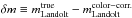 to be the difference between those two values. The calibration bias for SNe is given by the difference of δm for SNe and main sequence stars. Indeed the latter value sets the normalization of SN magnitudes through the assignement of a zero-point to the images. We label this difference Δm ≡ δm(SN) − δm(stars).
An uncertainty on the quantity Δm can be estimated by varying the SN model, the spectral library, or the filter transmissions. In practice, the uncertainty on the filter transmissions is dominant. Figure B.1 shows that δm is a function of the star color, which means that the filter model is inadequate. By construction, δm is color-independent for real observations. One can adjust wavelength shifts of the filter transmissions in order to obtain a color-independent value of δm for stars. This approach also results in a change of Δm that we can subsequently use as an estimate of the uncertainty due to approximate filter transmissions.
For the AndyCam CCD camera (CfA) with the Harris filter set (Harris et al. 1981), we have found ΔB = 0 ± 0.015 mag, ΔV = 0.03 ± 0.01 mag, and ΔR = 0.03 ± 0.03 mag. In other words, the color-correction does not significantly bias the measurements for the BVR bands. The situation for the U-band is, however, different. We have found a value as large as 0.1 for the 4Shooter camera (CfA), chip 1, with SAO filters. The values of δm for SNe and stars are represented in Fig. B.1 for this latter instrumental setup. One can also see on the figure that the residual color term is quite important. A U-band shift of ~3 nm is needed to obtain a flat distribution of δm, and in that case one finds an even larger value of ΔU = 0.15.
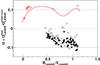 |
Fig. B.1
Synthetic values of |
| Open with DEXTER | |
A primary motivation for this study is the existence of significant calibration offsets between observer-frame UV observations from different instruments (see, e.g., Krisciunas et al. 2013, for a longer discussion of this effect) and with rest-frame UV observations at higher redshift. Kessler et al. (2009a) found that this latter discrepancy was responsible for a large part of the difference between the SALT2 and MLCS2k2 (Jha et al. 2007) models, MLCS2k2 being trained solely on low-z SNe. This U-band offset introduced by the application of a color-correction to SNe data could explain some of the discrepancy. However, the U-band filter transmissions are too uncertain to secure a good interpretation of natural magnitudes. For this reason, we adopt the magnitudes that are color-transformed to the Landolt system for the low-z samples (except for the CSP data and the CfA-III BVri light curves where we use the natural magnitudes and measured filter response functions), but assign a coherent systematic uncertainty of 0.1 mag to the amplitude of U-band light curves.
In all bands, the (phase dependent) error introduced by color transformations is not included, so measurement errors are typically underestimated. As a consequence, the uncertainties in the fit light-curve parameters are underestimated. The training of SALT2 is also affected by this problem. At present, we cannot afford discarding the color-transformed low-z and must deal with this issue. We estimate the measurement errors again for color transformed measurements in the low-z sample as follows. Since the SDSS-II and SNLS measurement errors are reliable, we trained a version of SALT2 as described in Sect. 4, but considering only the SNLS and SDSS-II measurements in the computation of the “error-snake”. We then use this version with reliable modeling of the intrinsic dispersion to fit all the color transformed low-z light curves. For each light-curve, we fit an ad-hoc two parameter (γ2 and γ3) correction of the measurement errors σi affecting the measurement di by minimizing the following residual likelihood: 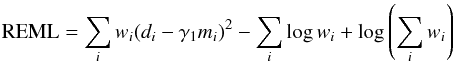 (B.1)with
 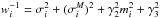 , where mi is the flux predicted by the best fit light-curve model and
  the model value of the intrinsic dispersion. We simultaneously fit for γ1, γ2 and γ3. When the light-curve contains less than five points, we fix the value of γ3 to zero. We then alter the errors in the light-curve accordingly to the fit values of γ2 and γ3. We found a mean value of 0.007 mag for γ2.
Appendix C: Estimates of missing host stellar masses in the C11 sample
The C11 compilation is missing estimates of the galaxy host mass for 61 nearby SNe (mostly because of missing photometry for the host). We describe estimates obtained for 57 of the 61 missing galaxy mass values.
For 49 of the nearby SN host galaxies, we derived an estimate based on Ks photometry (Bell & de Jong 2001; Bell et al. 2003) from the 2003 2MASS All-Sky Data Release of the Two Micron All Sky Survey (Skrutskie et al. 2006). The photometric data are extracted from the NASA/IPAC Extragalactic Database (NED) database. A linear model is fit between the mass and the Ks absolute magnitude on 51 objects with stellar mass estimates from C11. This linear model yields a residual of 0.15 dex and is used to provide galaxy mass estimates. For 8 galaxies without 2MASS Ks magnitudes, we rely on less precise models based on the total B band RC3 magnitude (de Vaucouleurs et al. 1991, three objects), the r C-Model magnitude (1 object from the SDSS DR6, Adelman-McCarthy et al. 2008), the B magnitude (three objects published in Hamuy et al. 2000), and the B magnitude in Strolger et al. (2002) for the low-luminosity host of SN 1999aw. The four remaining supernovae have no identified host and were assigned to the low-mass bin with an uncertainty on distance moduli of  added in quadrature to the other sources of uncertainty.
Appendix D: Accuracy of the CMB distance prior
In Sect. 7, we summarized the dark energy constraints from the CMB in the form of a distance prior. A computationally intensive, but more general, approach is to directly compare the CMB data to theoretical predictions for the fluctuation power spectra computed from a Boltzmann code. In this appendix, we briefly compare the results from both approaches for a fit of the w-CDM model to the combination of our SNe Ia JLA sample with CMB constraints.
The Planck collaboration (Planck collaboration XV 2014) has released code to compute the likelihood of theoretical models given Planck data22. This enables the marginalization of several sources of systematic uncertainty in the CMB spectra, such as errors in the instrumental beams and contamination by astrophysical foregrounds. In our comparison we make use of the full Planck temperature likelihood complemented with the WMAP measurement of the large scale CMB polarization (Bennett et al. 2013). We use the CAMB Boltzmann code (Lewis et al. 2000, March 2013) for our computation of CMB spectra. We follow assumptions from Planck Collaboration XVI (2014), fitting for the baryon density today ωb = Ωbh2, the cold dark matter density today ωc = Ωch2, θMC, the CosmoMC approximation of the sound horizon angular size computed from the Hu & Sugiyam (1996) fitting formulae, τ, the Thomson scattering optical depth due to reionization, ln(1010As), the log power of the primordial curvature perturbations at the pivot scale k0 = 0.05 Mpc-1, ns, the primordial spectrum index, and w, the dark energy equation of state parameter.
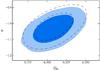 |
Fig. D.1
Comparison of two derivations of the 68 and 95% confidence contours in the Ωm and w parameters for a flat w-CDM cosmology. In one case, constraints are derived from the exploration of the full Planck+WP+JLA likelihood (blue). In the other case CMB constraints are summarized by the geometric distance prior described in Sect. 7.1 (dashed red). |
| Open with DEXTER | |
Best-fit parameters of the w-CDM fit for the full Planck+WP+JLA likelihood, and for the distance prior (DP+JLA).
We explored the Planck+WP+JLA likelihood with Markov chain Monte Carlo (MCMC) simulations of the posterior distribution assuming flat priors for parameters as given in Planck Collaboration XVI (2014, Table 1). Eight sample chains were drawn using CosmoMC (Lewis & Bridle 2002; Lewis 2013). Convergence of the simulation is monitored using the Gelman & Rubin (1992)R statistic23.
The mean value of the posterior distribution and 68% limits for the fit parameters to the Planck+WP+JLA likelihood are given in Table D.1. Best-fit parameters obtained using the distance prior in Sect. 7.2 are shown for comparison. The 68% and 95% contours from these simulations are drawn in Fig. D.1. Overplotted is the Planck+WP+JLA contour from Fig. 16. The differences are small as expected from the fact that the supplementary constraints brought by the complete CMB power spectrum are weak compared to the supernova constraints.
Appendix E: Compressed form of the JLA likelihood
Figure 9 shows that the correlation between the nuisance parameters (α, β, ΔM) and the cosmological parameter Ωm is small as a result of the high density of SNe in this Hubble diagram (especially in the SDSS sample at intermediate redshifts). This suggests that, for a limited class of models (those predicting isotropic luminosity distances evolving smoothly with redshifts), the estimate of distances can be made reasonably independent of the estimate of cosmological parameters. In this appendix, we seek to provide the cosmological information of the JLA Hubble diagram in a compressed form that is faster and easier to evaluate and still remains accurate for the most common cases. Studies investigating alternate cosmology or alternate standardization hypotheses for SNe-Ia should continue to rely on the complete form.
Appendix E.1: Binned distance estimates
The distance modulus is typically well approximated by a piece-wise linear function of log (z), defined on each segment zb ≤ z<zb + 1 as:  (E.1)with α = log (z/zb)/log (zb + 1/zb) and μb the distance modulus at zb. As an example, for 31 log-spaced control points zb in the redshift range 0.01 <z< 1.3, the difference between the Λ-CDM distance modulus and its linear interpolant is everywhere smaller than 1 mmag.
Such an interpolant can be fit to our measured Hubble diagram by minimizing a likelihood function similar to the one proposed in Eq. (15):  (E.2)The free parameters of the fit are α, β, ΔM and μb at the chosen control points. We use a fixed fiducial value of
  to provide uniquely determined μb. Results are compared to the best fit Λ-CDM cosmology in Fig. E.1. The structure of the correlation matrix of the best-fit μb is shown in Fig. E.2. It displays significant large scale correlation mostly due to systematic uncertainties. The tri-diagonal structure arises from the linear interpolation.
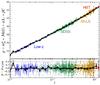 |
Fig. E.1
Binned version of the JLA Hubble diagram presented in Fig. 8. The binned points are solid circles. There are significant correlations between bins. The error bars are the square root of the diagonal of the covariance matrix given in Table F.2. |
| Open with DEXTER | |
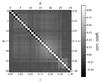 |
Fig. E.2
Correlation matrix of the binned distance modulus μb. |
| Open with DEXTER | |
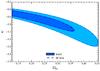 |
Fig. E.3
Comparison of the cosmological constraints obtained from the full JLA likelihood (filled contour) with approximate version derived by binning the JLA supernovae measurements in 20 bins (dashed blue contour) and 30 bins (continuous red contour). |
| Open with DEXTER | |
Appendix E.2: Cosmology fit to the binned distances
Cosmological models predicting isotropic luminosity distances evolving smoothly with redshifts can be fitted directly to the binned distance estimates. We denote DL(z;θ) the luminosity distance predicted by a model dependent of a set of cosmological parameters θ. A good approximation of the full JLA likelihood is generally given by the following likelihood function: 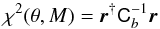 (E.3)with:
  (E.4)M a free normalization parameter, and Cb the covariance matrix of μb (see Table F.2). As an illustration, a comparison of the cosmological constraints obtained from the approximate and full version of the JLA likelihood for the w-CDM model is shown in Fig. E.3. For the models evaluated in Sect. 7 in combination with CMB and BAO constraints, the difference in best-fit estimates between the approximate and full version is at most 0.018σ and reported uncertainties differ by less than 0.3%.
We warn that the normalization parameter M must be left free in the fit and marginalized over when deriving uncertainties. Not doing so would be equivalent to introducing artificial constraints on the H0 parameter and would result in underestimated errors.
Appendix F: Data release
The light-curve fit parameters for the JLA sample are given in Table F.3. We provide the covariance matrices, described in Sect. 5.5, of statistical and systematic uncertainties in light-curve parameters. These two products contain all the information required to compute the likelihood function from Eq. (15) in a cosmological fit. We provide the necessary computer code in two forms: a CosmoMC plugin and an independent C++ code.
Alternatively, we deliver estimates of binned distance modulus μb obtained, as described in appendix E, for 31 control points
(30 bins) in Table F.1 and the associated covariance matrix in Table F.2. These values can be used to evaluate the approximate version of the JLA likelihood function proposed in Eq. (E.3).
In addition, we provide the retrained SALT2 model, the covariance matrix of calibration parameters, and the SNLS recalibrated light curves. The SDSS-II light curves can be obtained from the SDSS SN data release (Sako et al. 2014)24.
Binned distance modulus fitted to the JLA sample.
Covariance matrix of the binned distance modulus.
Parameters for the type Ia supernovae in the joint JLA cosmology sample.
© ESO, 2014
Current usage metrics show cumulative count of Article Views (full-text article views including HTML views, PDF and ePub downloads, according to the available data) and Abstracts Views on Vision4Press platform.
Data correspond to usage on the plateform after 2015. The current usage metrics is available 48-96 hours after online publication and is updated daily on week days.
Initial download of the metrics may take a while.