| Issue |
A&A
Volume 566, June 2014
|
|
|---|---|---|
| Article Number | A56 | |
| Number of page(s) | 17 | |
| Section | Astrophysical processes | |
| DOI | https://doi.org/10.1051/0004-6361/201423660 | |
| Published online | 11 June 2014 | |
Online material
Appendix A: Numerical implementation of the Hall effect
In this appendix, we provide details of the modifications made to the Pluto code (v4.0) to include the Hall effect. While these modifications are quite general to any conservative finite-volume numerical scheme, the interested reader would benefit by familiarising themselves with both Mignone et al. (2007) and the Pluto user manual.
Appendix A.1: Conservative finite-volume scheme
The implementation of Hall effect in Pluto has proven to be a difficult task. Our naive attempts to include the Hall effect as a source term in a way that is analogous to that used for Ohmic diffusion have failed. Since the Hall effect is in essence a dispersive term rather than a true diffusive term, we have instead incorporated the Hall effect into the heart of the conservative integration scheme.
We begin by writing Eqs. (1)–(3) in conservative form: 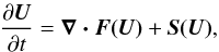 (A.1)where
U is a vector of conserved
quantities, F is the conservative flux function,
and S is the source term function. The
equations of isothermal Hall-MHD dictate
(A.1)where
U is a vector of conserved
quantities, F is the conservative flux function,
and S is the source term function. The
equations of isothermal Hall-MHD dictate 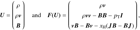 (A.2)where
 is the total pressure and
xH =
ηH/B
is the control parameter for the Hall effect.
is the total pressure and
xH =
ηH/B
is the control parameter for the Hall effect.
In the above formulation, we have explicitly used J = ∇×B in the flux function, which implies that the flux depends upon the conserved variables and their derivatives. This has dramatic consequences on the mathematical nature of the Riemann problem since it is ill-defined in this formulation (to wit, if B is discontinuous, then J is not defined). Another way to see this is to note that the linearised flux function, which defines the characteristic speeds of the system, depends upon the wavelength of the perturbation (due to the presence of whistler waves). If a discontinuity appears in the flow, one obtains infinitely fast characteristic speeds, which are, of course, unphysical.6 Because of this mathematical difficulty, we have not found any sensible way to derive accurate Riemann solvers, such as the Roe or HLLD solvers. Instead, we follow Tóth et al. (2008) and implement an HLL solver, which approximates the dynamics of Hall-MHD by assuming that J is an external parameter (i.e., not related to B). In doing so, we circumvent the difficulties exposed above at the expense of large numerical diffusivities.
The algorithm we designed to integrate Eqs. (A.1) and (A.2) using Pluto is as follows:
-
1.
Compute the primitive cell-averaged variables V from the conserved variables U.
-
2.
Reconstruct the primitive variables at the cell edges using a “well-chosen” second-order, total-variation-diminishing (TVD) spatial-reconstruction scheme (see below). This defines a left state (VL) and a right state (VR) at each cell face.
-
3.
Compute the left and right conserved variables UR /L from VR /L.
-
4.
Compute the face-centered J from the cell-averaged B using finite-difference formulae. Care is taken at this stage to apply the proper boundary conditions; shearing-sheet boundary conditions have to be applied explicitly to the currents to avoid spurious oscillations at radial boundaries due to interpolation errors.
-
5.
Compute the left and right fluxes using the left and right states and the face-centered current: FL/R = F(UL / R,J).
-
6.
Compute the Godunov flux F∗ using the whistler-modified HLL solver (described below).
-
7.
Evolve the conservative variables in time according to the equations of motion (see Mignone et al. 2007 for details). If constrained transport is used (Evans & Hawley 1988; Balsara & Spicer 1999), then the Godunov flux is used to compute the edge-centered electromotive forces (EMFs), which are then used to evolve the magnetic field.
To compute the Godunov flux F∗, we follow the HLL
scheme by using the approximation 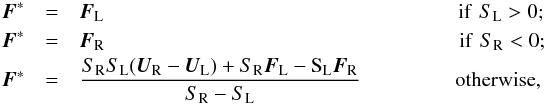 where
SL is the smallest algebraic signal
speed for the left state and SR is the largest algebraic signal
speed for the right state. Since we are solving the Hall-MHD equations,
SR
/L includes both the fast magnetosonic
speed and the whistler wave speed. Therefore, we choose
where
SL is the smallest algebraic signal
speed for the left state and SR is the largest algebraic signal
speed for the right state. Since we are solving the Hall-MHD equations,
SR
/L includes both the fast magnetosonic
speed and the whistler wave speed. Therefore, we choose
 where
v is
the flow speed, cf is the fast magnetosonic speed,
and cw is the whistler wave speed. As
whistler waves are dispersive, we choose cw to be equal to the whistler speed
at the grid scale:
where
v is
the flow speed, cf is the fast magnetosonic speed,
and cw is the whistler wave speed. As
whistler waves are dispersive, we choose cw to be equal to the whistler speed
at the grid scale: 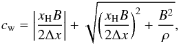 where
Δx is
the grid spacing in the direction under consideration.
where
Δx is
the grid spacing in the direction under consideration.
Appendix A.2: Numerical tests
Appendix A.2.1: Linear dispersion relation
We test our integration scheme by first considering a simple configuration with a uniform mean magnetic field B0 plus small sinusoidal perturbations δB⊥ perpendicular to B0. We then compute the frequency of the oscillation obtained in the code and compare it to the theoretical dispersion relation (see KL13 for details). The results are presented in Fig. A.1, where we have quantified the Hall effect by the Hall lengthscale ℓH and the Hall frequency ωH ≡ vA/ℓH.
In these numerical calculations, the Nyquist frequency is such that kℓH = 80. We find very good agreement for the whistler branch up to half of the Nyquist frequency. The non-propagating ion-cyclotron wave is not obtained at large k because of the large numerical dissipation: the dissipation rate of this wave is faster than its oscillation period.
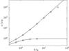 |
Fig. A.1
Dispersion relation for whistler waves. Black line: analytical prediction; circles: eigenfrequencies measured in Pluto using our implementation of the Hall effect. |
| Open with DEXTER | |
Numerical damping rate γ/ωH of a whistler wave as a function of the number of points per wavelength n using the monotonized centered (MC), Van Leer (VL), and minmod (MM) slope limiters.
Appendix A.2.2: Convergence and numerical dissipation
The question of convergence in Hall-MHD was raised by Tóth et al. (2008). Since the whistler wave speed ∝(dx)-1 and since numerical dissipation is roughly proportional to the wave speed, the convergence of the code at second order is not guaranteed in the presence of fast whistler waves. As was demonstrated by Tóth et al. (2008), this problem can be solved using a symmetric slope limiter in the reconstruction scheme, which naturally leads to a higher-order numerical diffusivity. To verify this, we present the numerical damping rate γ/ωH for a whistler wave at kℓH = 20 as a function of the number of points per wavelength n in Table A.1. We find that both the monotonized centered and Van Leer slope limiters show second-order convergence as the resolution per wavelength is increased. This is not the case for the minmod limiter, where only first-order convergence is obtained. These results support the Tóth et al. (2008) argument and demonstrate that great care is needed when choosing the slope limiter in Hall-MHD. Unless otherwise stated, we always use the monotonized centered slope limiter.
Tóth et al. (2008) also demonstrated that this algorithm leads to numerical dissipation ~cwU(4)(Δx)3, where U(n) stands for the nth derivative with respect to x. This implies that
-
numerical dissipation damps whistler waves at the grid scale in one oscillation period; this explains why it is not possible to measure the numerical eigenfrequency in Sect. A.2.1 at the Nyquist frequency;
-
at a given resolution, the damping rate decreases as k-4 (This has been verified by our numerical implementation.). Hence, numerical dissipation decreases very rapidly as one goes to larger scales.
Finally, KL13 have shown that higher-order time-integration schemes are one way to guarantee the stable propagation of whistler waves if one desires spectral accuracy without any numerical dissipation. Because of the numerical dissipation inherent to our algorithm, which is a natural consequence of the Godunov flux as defined above, the use of a higher-order time-integration scheme is not required in Pluto. We use an explicit second-order accurate Runge-Kutta scheme unless otherwise stated.
Appendix A.2.3: Unstratified shearing box
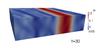 |
Fig. A.2
Snapshot of Bz in our unstratified Hall-MRI run at t = 30. The flow exhibits a zonal-field structure similar to that discovered by KL13. |
| Open with DEXTER | |
KL13 demonstrated that the Hall-dominated MRI with ⟨ By ⟩ ≲ ⟨ Bz ⟩ saturates by producing large-scale axisymmetric structures in the magnetic field (“zonal fields”). To further test our Hall-MHD integration scheme and to control our numerical diffusivity, we have tried to reproduce this non-linear behaviour in Pluto. We use very similar parameters to the run ZB1H1 of KL13. We use a 4 × 4 × 1 box with a resolution 64 × 64 × 16. We set ℓH = 0.55, Bz0 = 0.03, and η = ηA = 0. The resulting saturated state is shown in Fig. A.2 and exhibits a zonal-field structure similar to the one presented by KL13. This demonstrates that our scheme, despite being relatively diffusive due to the use of an HLL solver, manages to capture zonal-field structures with a resolution of 16 points per H.
Appendix B: Ambipolar diffusion
Ambipolar diffusion is implemented as a source term in a way analogous to that used for Ohmic resistivity. However, we noticed that grid-scale instabilities sometimes arise if the shearing-sheet boundary conditions are not enforced on the current density (a similar thing was observed with the Hall effect). Therefore, we use the current density computed in the conservative scheme for the Hall effect to compute the EMFs associated with ambipolar diffusion and Ohmic dissipation. This prevents small-scale instabilities from occurring at the radial boundaries.
We have tested our ambipolar diffusion module against the predictions of Kunz & Balbus (2004). An isothermal shearing box of size 4 × 4 × 1 and resolution 128 × 32 × 32 is threaded by a mean magnetic field with both vertical and horizontal components, whose magnitudes are characterised by their respective Alfvén speeds: Bz0 = 0.025 and By0 = 0.1. We introduce ambipolar diffusion by setting Am = 1. A typical snapshot of the linear growth phase is shown in Fig. B.1. We find the fastest-growing mode to have (kx,kz) = 2π × (−0.75,1). To check that this conforms to the expectation from linear theory, we show the theoretical growth rate of the ambipolar-dominated MRI as a function of (kx,kz) in Fig. B.2. We find that the mode seen in the simulation corresponds to the fastest-growing mode from linear theory that is available in the simulation. The theoretical growth rate for this mode is γ = 0.171; we find numerically γ = 0.17. This demonstrates the accuracy of our implementation of ambipolar diffusion in Pluto.
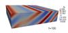 |
Fig. B.1
Snapshot of Bx in our ambipolar-MRI test simulation at t = 100, just before saturation. The oblique nature of MRI channel mode, as predicted by Kunz & Balbus (2004), is evident. |
| Open with DEXTER | |
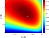 |
Fig. B.2
Growth rate of the ambipolar-MRI for Bz0 = 0.025 and By0 = 0.1 as a function of the horizontal and vertical wavenumbers, kx and kz. The largest growth rate available in the simulation obtains for (kx,kz) = 2π × (−0.75,1) (white cross). |
| Open with DEXTER | |
© ESO, 2014
Current usage metrics show cumulative count of Article Views (full-text article views including HTML views, PDF and ePub downloads, according to the available data) and Abstracts Views on Vision4Press platform.
Data correspond to usage on the plateform after 2015. The current usage metrics is available 48-96 hours after online publication and is updated daily on week days.
Initial download of the metrics may take a while.