Accelerated post-AGB evolution, initial-final mass relations, and the star-formation history of the Galactic bulge

Home

All issues

Volume 566 (June 2014)

A&A, 566 (2014) A48

Online Material

Free Access

Issue		A&A Volume 566, June 2014


Article Number		A48
Number of page(s)		27
Section		Interstellar and circumstellar matter
DOI		https://doi.org/10.1051/0004-6361/201118391
Published online		11 June 2014

Online material

Appendix A: Observations and models of planetary nebulae

The model fitting procedure was described in brief in Sect. 2.3. A full description can be found in Gesicki et al. (2006), where we applied a genetic algorithm for the first time to locate the best fit parameters.

We searched for the density and velocity distributions as simply as possible. The density was assumed similar to a reversed parabola with both edges modified to fit the images. The best fit was judged by visual inspection of the superposed images shown below in the boxes marked “surface brightness”. The stellar temperature, luminosity, and the ionized mass was derived by PIKAIA as a compromise to a simultaneously satisfying fit to all available emission strengths (see Table A.1). The density values at the innermost and outermost edges were additionally modified to reproduce the strengths of emissions originated there, but the velocity field was solely derived by the PIKAIA routine, which

judges the results by the quality of emission profile fitting (least squares method). The best velocity field was searched among linear or parabola shapes. More complicated velocity fields were not considered. Wherever the parabola provided no improvement of the fit, we adopted the linear velocity as the simplest.

This method was applied identically for all 31 objects presented below. The largest nebulae and those barely resolved are treated in the same way to allow us to discuss the whole data set consistently.

The series of figures (Figs. A.1–A.31, one per object) present the HST observations with the derived model dependencies. The HST image are shown rotated, such that the VLT echelle spectroscopic slit is horizontal. In most cases, this puts the slit along the minor axis of the PN. The echelle spectrum was extracted from the central arcsecond only. For extended objects, outer areas of the slit were not used. Wherever no observational data was available, we left the corresponding box empty.

Table A.1

GB PNe observed Hβ fluxes and line strengths together with the corresponding photoionization model results.

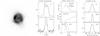Fig. A.1

Nebula H 1-55 (PN G 001.7−04.4). The left panel shows the HST Hα image in linear grey scale, which is rotated so that the VLT spectrograph slit runs horizontally through the centre. In the small panels, the observed data are drawn in solid lines (as a rule), while model fits and model parameters are in dotted and dashed lines. The “surface brightness” panel shows the horizontal slices through the Hα and [O iii] image centre (averaged over nine pixels) with the model brightness profile superposed. Next, the radial distributions of the best-fit model for selected parameters are shown. The right-most panel shows the emission lines observed at the VLT with the superposed modelled line profiles corrected for instrumental broadening of 0.1 Å.

Open with DEXTER

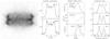	Fig. A.2 Nebula H 2-37 (PN G 002.3−03.4). The data are presented as in Fig. A.1.
Open with DEXTER

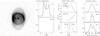	Fig. A.3 Nebula H 2-20 (PN G 002.8+01.7). The data are presented as in Fig. A.1.
Open with DEXTER

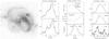	Fig. A.4 Nebula H 2-39 (PN G 002.9-03.9). The data are presented as in Fig. A.1. In spite of the complex structure, the velocity profile is well reproduced by the 1D model.
Open with DEXTER

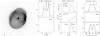	Fig. A.5 Nebula H 2-17 (PN G 003.1+03.4). The data are presented as in Fig. A.1.
Open with DEXTER

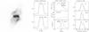	Fig. A.6 Nebula M 2-14 (PN G 003.6+03.1). The data are presented as in Fig. A.1. The slit is along the minor axis. The high velocity wing of the [N ii] line is not in the model (which assumes a linear velocity gradient). It may arise from the base of the polar flow.
Open with DEXTER

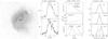	Fig. A.7 Nebula H 2-15 (PN G 003.8+05.3). The data are presented as in Fig. A.1.
Open with DEXTER

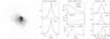	Fig. A.8 Nebula KFL 11 (PN G 004.1−03.8). The data are presented as in Fig. A.1. The [N ii] profile is one sided, indicating an asymmetry in the nebula, which is also evident from the image. However, the velocity field is well fitted.
Open with DEXTER

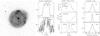	Fig. A.9 Nebula H 2-25 (PN G 004.8+02.0). The data are presented as in Fig. A.1.
Open with DEXTER

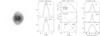	Fig. A.10 Nebula M 1-20 (PN G 006.1+08.3). The data are presented as in Fig. A.1.
Open with DEXTER

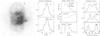	Fig. A.11 Nebula H 2-18 (PN G 006.3+04.4). The data are presented as in Fig. A.1.
Open with DEXTER

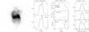	Fig. A.12 Nebula M 1-31 (PN G 006.4+02.0). The data are presented as in Fig. A.1.
Open with DEXTER

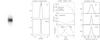	Fig. A.13 Nebula He 2-260 (PN G 008.2+06.8). The data are presented as in Fig. A.1.
Open with DEXTER

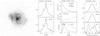	Fig. A.14 Nebula MaC 1-11 (PN G 008.6−02.6). The data are presented as in Fig. A.1. The [N ii] line shows a velocity asymmetry, which may also be just visible in [O iii]. The model fits the red-shifted velocities.
Open with DEXTER

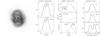	Fig. A.15 Nebula M 1-19 (PN G 351.1+04.8). The data are presented as in Fig. A.1.
Open with DEXTER

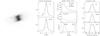	Fig. A.16 Nebula Wray 16-286 (PN G 351.9-01.9). The data are presented as in Fig. A.1. The slit was oriented along the major axis.
Open with DEXTER

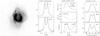	Fig. A.17 Nebula H 1-8 (PN G 352.6+03.0). The data are presented as in Fig. A.1.
Open with DEXTER

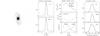	Fig. A.18 Nebula Th 3-4 (PN G 354.5+03.3). The data are presented as in Fig. A.1.
Open with DEXTER

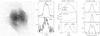	Fig. A.19 Nebula Th 3-6 (PN G 354.9+03.5). The data are presented as in Fig. A.1.
Open with DEXTER

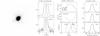	Fig. A.20 Nebula H 1-9 (PN G 355.9+03.6). The data are presented as in Fig. A.1. The radial profile is shown scaled by a factor of 100. The nebula is very compact and the model does not fit the radial distribution well, but the outer radius of the model closely aligns with the edge of the image, as seen in the figure.
Open with DEXTER

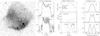	Fig. A.21 Nebula H 2-26 (PN G 356.1-03.3). The data are presented as in Fig. A.1.
Open with DEXTER

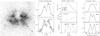	Fig. A.22 Nebula H 2-27 (PN G 356.5-03.6). The data are presented as in Fig. A.1.
Open with DEXTER

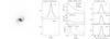	Fig. A.23 Nebula Th 3-12 (PN G 356.8+03.3). The data are presented as in Fig. A.1. The very compact nebula shows a spiral-like structure, likely tracing a bipolar flow. The profiles do not show evidence for high-velocity flows and are well fitted.
Open with DEXTER

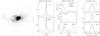	Fig. A.24 Nebula M 3-38 (PN G 356.9+04.4). The data are presented as in Fig. A.1. The slit is oriented along the major axis.
Open with DEXTER

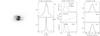	Fig. A.25 Nebula H 1-43 (PN G 357.1-04.7). The data are presented as in Fig. A.1.
Open with DEXTER

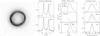Fig. A.26

Nebula H 2-13 (PN G 357.2+02.0). The data are presented as in Fig. A.1. The morphology is deceptively simple but the velocity profile, especially in [O iii], is complex and the [O iii] line is (unusually) wider than [N ii]. Note that the profile is extracted from the inner arcsecond and not from the bright rim. This may be a bipolar nebula seen pole-on with polar flows contributing to the line broadening.

Open with DEXTER

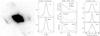	Fig. A.27 Nebula H 1-46 (PN G 358.5−04.2). The data are presented as in Fig. A.1. The slit is oriented along the major axis.
Open with DEXTER

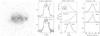	Fig. A.28 Nebula Al 2-F (PN G 358.5+02.9). The data are presented as in Fig. A.1. A quadrupolar nebula.
Open with DEXTER

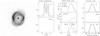	Fig. A.29 Nebula M 3-40 (PN G 358.7+05.2). The data are presented as in Fig. A.1.
Open with DEXTER

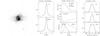	Fig. A.30 Nebula H 1-19 (PN G 358.9+03.4). The data are presented as in Fig. A.1. The slit is oriented along the major axis.
Open with DEXTER

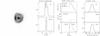	Fig. A.31 Nebula Th 3-14 (PN G 359.2+04.7). The data are presented as in Fig. A.1. There is no [O iii] detected: the spatial profile appears to show stellar continuum only.
Open with DEXTER

© ESO, 2014

Current usage metrics show cumulative count of Article Views (full-text article views including HTML views, PDF and ePub downloads, according to the available data) and Abstracts Views on Vision4Press platform.

Data correspond to usage on the plateform after 2015. The current usage metrics is available 48-96 hours after online publication and is updated daily on week days.

Initial download of the metrics may take a while.