| Issue |
A&A
Volume 565, May 2014
|
|
|---|---|---|
| Article Number | A76 | |
| Number of page(s) | 19 | |
| Section | Stellar structure and evolution | |
| DOI | https://doi.org/10.1051/0004-6361/201220507 | |
| Published online | 14 May 2014 | |
Online material
Appendix A: Details about Kurucz’s and K-OPAL opacity data
Examples of Meszaros et al. (2012) opacity data available from ATLAS-APOGEE website.
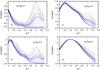 |
Fig. A.1
Rosseland-mean opacities lgκR [ cm2 g-1 ] calculated by Castelli & Kurucz for different chemical composition of elements and ξ = 0. The data plotted for the gas pressure, lgPg = 2,4,6, and 8 (in cgs units) were taken from the Castelli website on 2012. Black lines show opacity data Nos. 1–9 listed in Table A.1, while blue lines display opacity data Nos. 10–22. |
| Open with DEXTER | |
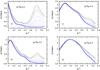 |
Fig. A.2
Same as Fig. A.1, but the Rosseland-mean opacities lgκR [ cm2 g-1 ] calculated by Castelli & Kurucz for enhanced abundances of O, Ne, Mg, Si, S, Ar, Ca, and Ti elements by +0.4 dex, viz., opacity data Nos. 23–35 listed in Table A.1 were plotted. |
| Open with DEXTER | |
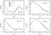 |
Fig. A.3
Examples of the Rosseland-mean opacities lgκR [ cm2 g-1 ] calculated by Meszaros et al. for different chemical composition of elements and ξ = 2km s-1 (Table A.2). The data plotted for the gas pressure, lgPg = 2,4,6, and 8 (in cgs units) were taken from the ATLAS-APOGEE website on 2013. |
| Open with DEXTER | |
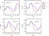 |
Fig. A.4
Derivatives of the Rosseland-mean opacities over density
|
| Open with DEXTER | |

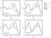 |
Fig. A.5
Same as Fig. A.4, but for |
| Open with DEXTER | |

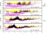 |
Fig. A.6
OP monochromatic cross-sections lgσ (in atomic units) vs.
|
| Open with DEXTER | |

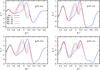 |
Fig. A.7
Derivatives of the Rosseland-mean opacities over temperature
|
| Open with DEXTER | |

The Rosseland-mean opacities calculated by Castelli & Kurucz are available in tabular form for different metallicities and microturbulent velocities ξ = 0,1,2,4, and 8 km s-1. Following Kurucz, the data (Table A.1) were named using the scheme, which describes abundances of metals relative to the solar abundances listed in Grevesse & Sauval (1998). In particular, p15 corresponds to enhanced abundances of metals by [m/H] = lg(m/H) − lg(m/H)⊙ = +1.5 dex, the solar chemical composition ([m/H] = +0.0) is denoted as p00, and [m/H] = −4.0 as m40. The X, Y, and Z abundance parameters and the mass abundances of oxygen (ZO) and iron (ZFe) were also shown in Table A.1. The opacity data Nos. 1–22 have the same relative abundances of metals taken from Grevesse & Sauval (1998), while data Nos. 23–35 have enhanced abundances of O, Ne, Mg, Si, S, Ar, Ca, and Ti by +0.4 dex. These elements are produced by stellar nucleosyntheses in the α-process. The last two rows in Table A.1 show the abundance parameters listed in Asplund et al. (2005) and Asplund et al. (2009).
The CK Rosseland-mean opacities,  , were
tabulated for 3.3 ≤ lgT ≤
5.3 and −4.0 ≤
lgPg ≤ 8.0, where Pg is the gas
pressure in the cgs units. Figure A.1 shows
, were
tabulated for 3.3 ≤ lgT ≤
5.3 and −4.0 ≤
lgPg ≤ 8.0, where Pg is the gas
pressure in the cgs units. Figure A.1 shows  as a
function of lgT for lgPg =
2,4,6, and 8, and ξ = 0. In each panel, the
top line corresponds to X =
0.4786 and Z = 0.3596, while the bottom line to
X =
0.7474 and Z = 1.49 × 10⁻⁷ (Table A.1). Clearly, the opacity bump at lgT ≈ 5.06 is caused by
metals and can be explained by much more detailed atom models of the new Kurucz data.
The opacities with enhanced abundances of the α-rich elements (O, Ne, Mg, Si, S, Ar, Ca, and
Ti) by +0.4 dex. were plotted in Fig. A.2. These elements participate in the opacity
bump at lgT ≈
5.06 in addition to other heavy elements (cf. also Fig. 2, where the data of m05 and m05a
were plotted).
as a
function of lgT for lgPg =
2,4,6, and 8, and ξ = 0. In each panel, the
top line corresponds to X =
0.4786 and Z = 0.3596, while the bottom line to
X =
0.7474 and Z = 1.49 × 10⁻⁷ (Table A.1). Clearly, the opacity bump at lgT ≈ 5.06 is caused by
metals and can be explained by much more detailed atom models of the new Kurucz data.
The opacities with enhanced abundances of the α-rich elements (O, Ne, Mg, Si, S, Ar, Ca, and
Ti) by +0.4 dex. were plotted in Fig. A.2. These elements participate in the opacity
bump at lgT ≈
5.06 in addition to other heavy elements (cf. also Fig. 2, where the data of m05 and m05a
were plotted).
Recently, an extensive grid of atmosphere models, as well as the Rosseland-mean
opacities,  , were
recalculated by Meszaros et al. (2012) for scaled
solar abundances of metals given by Asplund et al. (2005). Examples are shown in Table A.2
and Fig. A.3. The data were named using the Kurucz scheme for the scaled metal
(m)
abundances composed with a standard/nonstandard content of C (c) and O (o).
, were
recalculated by Meszaros et al. (2012) for scaled
solar abundances of metals given by Asplund et al. (2005). Examples are shown in Table A.2
and Fig. A.3. The data were named using the Kurucz scheme for the scaled metal
(m)
abundances composed with a standard/nonstandard content of C (c) and O (o).
We would like to note that Castelli & Kurucz’s mixture of elements has higher values of Z and ZO than those of Asplund et al. (2009), but the same abundance of Fe. The Meszaros et al. data (M) have lower Z- and ZFe-values. In addition, the helium abundance of the CK and M standard (solar) mixtures is not far from the helioseismological value Y = 0.2485 given by Basu & Antia (2004). This helium abundance was adopted by Grevesse & Sauval (1998), Asplund et al. (2005) and Asplund et al. (2009). The CK and M elemental mixtures have Y = 0.1635−0.2526 (Tables A.1 and A.2).
The CK and M atmosphere models are available from Castelli and ATLAS-APOGEE websites (Sect. 3), respectively. The older models, available from Kurucz website, were calculated for older opacity distribution functions (ODF) with about 58 million lines of atoms and molecules in total. Despite this, according to Kurucz (2011), the line opacity was underestimated because not enough lines were included in calculations.
According to Kurucz (2012, priv. comm.), the CK opacities are less reliable for
lgT ≥
5.2. The K-OPAL models were therefore calculated using the CK (or M)
opacities for lgT < 5.2 and the OPAL (or
OP) data for higher temperatures. We adjusted these two kinds of Rosseland-mean
opacities at lgT =
5.2, assuming  . The opacity data are
usually included as tables of κR(lgT,lgR)
(the OPAL format) in computing codes for modeling stellar structure, where
lgR = lgρ
− 3lgT + 18. We attempted to achieve good accuracy
in the transformation of κR from (lgT,lgPg) to
(lgT,lgR) variables. First, we
solved the EOS with a Kurucz’s computing code to find out gas densities, ρ, for each pair of
(lgT,
lgPg). Next, we interpolated the opacity
data to (lgT, lgR)-points. In addition to κR, the
derivatives of the Rosseland-mean opacities over temperature and density were calculated
numerically with two methods. In the first method, having already calculated tables of
κR(lgT,lgρ),
we used Kurucz’s (1970) differentiation procedure
to obtain
. The opacity data are
usually included as tables of κR(lgT,lgR)
(the OPAL format) in computing codes for modeling stellar structure, where
lgR = lgρ
− 3lgT + 18. We attempted to achieve good accuracy
in the transformation of κR from (lgT,lgPg) to
(lgT,lgR) variables. First, we
solved the EOS with a Kurucz’s computing code to find out gas densities, ρ, for each pair of
(lgT,
lgPg). Next, we interpolated the opacity
data to (lgT, lgR)-points. In addition to κR, the
derivatives of the Rosseland-mean opacities over temperature and density were calculated
numerically with two methods. In the first method, having already calculated tables of
κR(lgT,lgρ),
we used Kurucz’s (1970) differentiation procedure
to obtain  and
and
 .
Next, we used the thermodynamic identity for
.
Next, we used the thermodynamic identity for
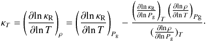 (A.1)Again,
the CK (or M) and OPAL (or OP) derivatives were adjusted at lgT = 5.2. In the second
method, we started from κR(lgT,lgR)
and ran Seaton’s (1993) bicubic interpolation
procedure, which involves 16 neighborhood points as well as the derivatives of
κR over temperature and density. Both
methods yield similar results, although the second method reveals a little bit more
regular behavior of the derivatives because of the higher number of data points involved
in the procedure. In the rest of this paper we used data obtained from the second
method. No additional smoothing procedure was ran.
(A.1)Again,
the CK (or M) and OPAL (or OP) derivatives were adjusted at lgT = 5.2. In the second
method, we started from κR(lgT,lgR)
and ran Seaton’s (1993) bicubic interpolation
procedure, which involves 16 neighborhood points as well as the derivatives of
κR over temperature and density. Both
methods yield similar results, although the second method reveals a little bit more
regular behavior of the derivatives because of the higher number of data points involved
in the procedure. In the rest of this paper we used data obtained from the second
method. No additional smoothing procedure was ran.
The K-OPAL opacity data discussed in Sect. 3 show two opacity bumps at lgT = 5.06 and
5.3. Examples of the
hybrid opacities, κR were plotted in Fig. 2 and their derivatives over density, (κρ)T,
and temperature (κT)ρ,
in Figs. A.4 and A.5, respectively. The local minimum of the opacity at lgT = 5.2 plays a crucial
role in the K-OPAL seismic models of B stars as discussed in Sect. 5. A deeper insight
into the problem follows from an analysis of the OP monochromatic opacities. Figure A.6
shows contributions of different elements to the total opacity (yellow lines) for
lgT =
4.8,5.0, and 5.3, and lgNe = 16. The
black lines display opacity caused by H, He, Fe, and electron scattering
(σe), while cross-sections of Fe are
shown as violet lines. In Fig. A.6, the monochromatic cross-sections, σ(u) are
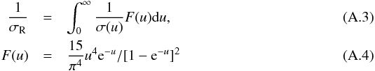
given in atomic units, where  .
The Rosseland-mean opacity per unit mass is then
.
The Rosseland-mean opacity per unit mass is then
 (A.2)where
 and
μ is the
mean atomic weight. The smooth red lines in Fig. A.6, corresponding to lgF(u) +
C, display that a spectral region near
u = 3.83
contributes mostly to the Rosseland-mean opacity. The constant C was introduced for
better visibility of the Rosseland-mean weighting function (corrected for stimulated
emission), F(u). In the cases of
lgT = 4.8
and 5.0, the Fe-curtain (violet lines in Fig. A.6) is located well below opacity caused
by H, He, and σe at spectral region near
u ≈ 3.83.
Note that the contribution of metals other than Fe is significant at lgT = 5.0. This is the
reason why the new Kurucz data were able to change the Rosseland-mean opacity mostly
near lgT =
5.06. The Fe-curtain dominates at lgT = 5.3 (Fig. A.6).
Now, the OP (and OPAL) opacity is caused mostly by very many lines due to Fe in electron
configurations of the type 3sx3py3dz and
3sx3py3dznl, (Iglesias et al.
1990; Lynas-Gray et al. 1995; Seaton et al. 1994). As
one can see, the synthetic Fe cross-section is located above the total cross-sections
caused by H, He, and σe (a brown line) near u ≈ 3.83 (and
u ≥ 7).
This changes quickly depending on the temperature. At lgT = 5.2, the Fe-curtain
is also seen, but its maximum is shifted to u ≈ 5. Similarly, the maximum is located at
u ≈ 2.3
for lgT =
5.5. As a result, the OP (and OPAL) opacity bump at lgT = 5.3 is narrow and
the K-OP (and K-OPAL) data have a two-peak structure of κR with the
additional opacity bump at lgT = 5.06.
and
μ is the
mean atomic weight. The smooth red lines in Fig. A.6, corresponding to lgF(u) +
C, display that a spectral region near
u = 3.83
contributes mostly to the Rosseland-mean opacity. The constant C was introduced for
better visibility of the Rosseland-mean weighting function (corrected for stimulated
emission), F(u). In the cases of
lgT = 4.8
and 5.0, the Fe-curtain (violet lines in Fig. A.6) is located well below opacity caused
by H, He, and σe at spectral region near
u ≈ 3.83.
Note that the contribution of metals other than Fe is significant at lgT = 5.0. This is the
reason why the new Kurucz data were able to change the Rosseland-mean opacity mostly
near lgT =
5.06. The Fe-curtain dominates at lgT = 5.3 (Fig. A.6).
Now, the OP (and OPAL) opacity is caused mostly by very many lines due to Fe in electron
configurations of the type 3sx3py3dz and
3sx3py3dznl, (Iglesias et al.
1990; Lynas-Gray et al. 1995; Seaton et al. 1994). As
one can see, the synthetic Fe cross-section is located above the total cross-sections
caused by H, He, and σe (a brown line) near u ≈ 3.83 (and
u ≥ 7).
This changes quickly depending on the temperature. At lgT = 5.2, the Fe-curtain
is also seen, but its maximum is shifted to u ≈ 5. Similarly, the maximum is located at
u ≈ 2.3
for lgT =
5.5. As a result, the OP (and OPAL) opacity bump at lgT = 5.3 is narrow and
the K-OP (and K-OPAL) data have a two-peak structure of κR with the
additional opacity bump at lgT = 5.06.
As mentioned in Sect. 3.2, the K-OPAL/B models were designed to study how the relative
strength of the opacity bumps at lgT = 5.06 and 5.3 influence seismic models of
early-type stars. They are basically the OPAL models for Z = 0.0264 and
Z =
0.0168, but  was selected near the opacity
bump at lgT ≈
5.06. The CK opacity data of m075,m05,m04,m02,
and p00
were considered. Figures A.7 show κR and κT for models
of Nos. 18–20 (Table 1) in comparison with the
OPAL (No. 1) and K-OPAL/A data (No. 11).
was selected near the opacity
bump at lgT ≈
5.06. The CK opacity data of m075,m05,m04,m02,
and p00
were considered. Figures A.7 show κR and κT for models
of Nos. 18–20 (Table 1) in comparison with the
OPAL (No. 1) and K-OPAL/A data (No. 11).
Relatively little is known about the sensitivity of the OP and OPAL data to the pressure-broadening parameters for spectral lines. There is little sensitivity at high densities, where the lines become very broad and give a quasicontinuum, or at very low densities, where the profiles are mainly determined by Doppler broadening and radiation damping. At intermediate densities, like lgNe = 15.5 and lgT = 5.2 (lgR = −5.8) discussed by Seaton et al. (1994), an increase of the pressure broadening parameters of Fe lines by a factor of 2 results in an increase in the Rosseland-mean opacity by 33 per cent for the solar mix of elements. The opacity is much lower when only doppler broadening of lines is assumed (Rogers & Iglesias 1992).
In addition, including more electron configurations and many more line transitions, as in Kurucz (2011), would probably also increase opacity at lgT> 5.2. Another potentially important reason why the OP (and OPAL) opacities should be upgraded is related to autoionizing transitions. In the OP project, these transitions were treated as resonances in photoionization cross-sections (Bautista 1997). To make the problem tractable, each LS-term was represented by only one level with its average energy. The splitting of spectroscopic LS terms
into individual levels may be necessary for final calculations of photoionization cross-sections with resonance structures. This is suggested by Kurucz’s treatment of autoionizing transitions (Castelli & Kurucz 2004) and by recent results published by Nahar et al. (2011), which include the fine structure explicitly for Fe XVII. Similarly, the new effective cross-sections with photoexcitation-of-core (PEC) resonances for O III and Fe XXI are much higher, up to two orders of magnitude, than in the OP data (Fig. 1 in Pradhan & Nahar 2009). The missing opacity in the OP data may lie in an energy range from a few eV to few hundreds of eV, depending on the element and ionization stage. Therefore, we also searched K-OPAL/C (and K-OP/C) models (with opacity data Nos. 23–25) with enhanced opacities at lgT> 5.2. In the case of No. 23, EOS and nuclear reaction rates were calculated for the initial (at ZAMS) chemical composition of X = 0.7394, Y = 0.2499, and Z = 0.0107. The CK opacity data corresponding to Z = 0.0107 were assumed at lgT < 5.2, but the OPAL opacities corresponding to Z = 0.0264 at lgT> 5.2. Similarly, models of Nos. 24 and 25, were calculated for Z = 0.00537 and 0.00303 with enhanced opacities at lgT> 5.2 (OPAL: Z = 0.0168 and 0.0134), respectively.
Examples of κR and κT are shown in Figs. 11 and 12 (Sect. 5), where differential work integrals were plotted for the K-OPAL models.
© ESO, 2014
Current usage metrics show cumulative count of Article Views (full-text article views including HTML views, PDF and ePub downloads, according to the available data) and Abstracts Views on Vision4Press platform.
Data correspond to usage on the plateform after 2015. The current usage metrics is available 48-96 hours after online publication and is updated daily on week days.
Initial download of the metrics may take a while.