| Issue |
A&A
Volume 564, April 2014
|
|
|---|---|---|
| Article Number | A21 | |
| Number of page(s) | 14 | |
| Section | Interstellar and circumstellar matter | |
| DOI | https://doi.org/10.1051/0004-6361/201323170 | |
| Published online | 28 March 2014 | |
Online material
Appendix A: Channel maps
The proper channel maps of the two ammonia lines observed are presented in Figs. A.1 and A.2. The collection of spectra are also available at the CDS.
 |
Fig. A.1
Channel maps of the NH3 (1, 1) emission. Only the main hyperfine component is depicted. LSR velocities are indicated at the top centre of each map. Contours are 0.15, 0.30, 0.45, 0.60, 0.90, 1.20, 1.50, 1.80, 2.25, 2.70, 3.15, 3.60, 4.20, and 4.8 K. |
| Open with DEXTER | |
 |
Fig. A.2
Channel maps of the NH3 (2, 2) emission. Only the main hyperfine component is depicted. LSR velocities are indicated at the top centre of each map. Contours are 0.18, 0.36, 0.54, 0.72, and 1.08 K. |
| Open with DEXTER | |
Appendix B: Formulation
In this Appendix we summarize the formulae used to determine some physical properties (opacities, rotational temperatures, column densities, and abundances) from the observed NH3 lines. This corresponds to the standard interpretation previously discussed and presented by several authors, such as Ungerechts et al. (1986) and Busquet et al. (2009).
Appendix B.1: Hyperfine and Gaussian fitting
The NH3 lines are split by the quadrupole hyperfine interaction (Ho & Townes 1983). From the relative intensities of the main hf group and the four satellite ones, it is possible to directly derive the optical depth of the main hf group (Pauls et al. 1983). When the satellite (1, 1) lines were detected, a CLASS method was used for this fitting. The output is: (1) A τm = f [Jν(Texc) − Jν(Tbg)] τm; (2) LSR velocity (VLSR); (3) line width at half maximum (Δv); and (4) τm, the opacity of the main hf group. f is the beam-filling factor, and Jν(T) is Rayleigh-Jeans temperature, defined as Jν(T) = (h ν/k) (eh ν/k T − 1)-1, Tbg = 2.73 K is the background temperature, and h and k are the Planck and Boltzmann constants, respectively.
This formulation assumes that all the hf levels are populated according to local
thermodynamic equilibrium (LTE) conditions, and a Gaussian velocity distribution. The
level population is characterized by the excitation temperature Texc, which
can be cleared from the fitting by
 (B.1)where
W = Jν(Texc) = A/f + Jν(Tbg).
(B.1)where
W = Jν(Texc) = A/f + Jν(Tbg).
The column density of a NH3(J,K) level, N(J,K), is obtained by
 (B.2)where
ν is
the line frequency in GHz, τtot is the “total” opacity of all
the hf components, and Δv and Texc are in km s-1 and K, respectively. The
above equation results from solving the transport equation for the NH3 molecule (Wilson et al. 2009), using a dipole moment
μ = 1.469 D, and assuming Texc≫Tbg.
(B.2)where
ν is
the line frequency in GHz, τtot is the “total” opacity of all
the hf components, and Δv and Texc are in km s-1 and K, respectively. The
above equation results from solving the transport equation for the NH3 molecule (Wilson et al. 2009), using a dipole moment
μ = 1.469 D, and assuming Texc≫Tbg.
When hyperfine fitting was possible, we estimated the column density of the (1, 1)
level, N(1, 1), using the above equation. Numerically, it
is computed by  (B.3)where
a rough assumption of τtot = 2 τm
was used.
(B.3)where
a rough assumption of τtot = 2 τm
was used.
When hyperfine fitting was not possible, we assumed optically thin emission. In this
case, Eq. (B.2) for the (1, 1) line results in
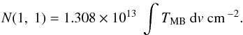 (B.4)In
the above equation, all the hf components are included in the integral. If the
integration only extends to the main group, the coefficient needs to be multiplied by
a factor of 2.
(B.4)In
the above equation, all the hf components are included in the integral. If the
integration only extends to the main group, the coefficient needs to be multiplied by
a factor of 2.
In the case of the (2, 2) line, the equivalent expression is
 (B.5)Provided
N(1, 1) and N(2,2), the rotational temperature
Trot can be computed (Townes & Schawlow 1975; Ho & Townes 1983) by
(B.5)Provided
N(1, 1) and N(2,2), the rotational temperature
Trot can be computed (Townes & Schawlow 1975; Ho & Townes 1983) by
 (B.6)which
results from a two-level system approximation (Ho
& Townes 1983).
(B.6)which
results from a two-level system approximation (Ho
& Townes 1983).
The partition function is given by
 (B.7)where
gJK = (2J + 1) gop
and EJK are the
statistical weight and the energy of the level (J,K), and
gop is the statistical weight for the
ortho and para species. In the above equation we summed to the first four levels3 and assumed that (1) only the metastable levels are
populated; (2) the levels are characterized by the LTE temperature T; and (3)
gop equals to 2 and 1 for the ortho
and para species, respectively.
(B.7)where
gJK = (2J + 1) gop
and EJK are the
statistical weight and the energy of the level (J,K), and
gop is the statistical weight for the
ortho and para species. In the above equation we summed to the first four levels3 and assumed that (1) only the metastable levels are
populated; (2) the levels are characterized by the LTE temperature T; and (3)
gop equals to 2 and 1 for the ortho
and para species, respectively.
The total column density of all the metastable lines may be computed from a single
line and by assuming a partition function characterized by T = Trot (e.g.
Ungerechts et al. 1986; Busquet et al. 2009):
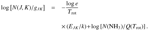
 (B.8)In
particular, for the (1, 1) line the above equation becomes
(B.8)In
particular, for the (1, 1) line the above equation becomes
 (B.9)When
the (2, 2) line is the only one detected, an equivalent formula to (B.9) is
(B.9)When
the (2, 2) line is the only one detected, an equivalent formula to (B.9) is
 (B.10)
Appendix B.2: Abundances
The NH3
abundance is computed by  (B.11)where
N(H2) is the H2 column density. To estimate it, we used the survey
of the Cygnus region conducted by Motte et al.
(2007) in the 1.2 mm continuum emission.
(B.11)where
N(H2) is the H2 column density. To estimate it, we used the survey
of the Cygnus region conducted by Motte et al.
(2007) in the 1.2 mm continuum emission.
At this wavelength, most of the flux arises from thermal dust emission, which is optically thin. By assuming a constant gas-to-dust ratio, the 1.2 mm flux is directly related to the total amount of molecular gas. We therefore used the formulation of Motte et al. (1998), adapted to our case.
More precisely, we used their Eq. (1), which computes N(H2) as a function of the 1.2 mm flux, the dust temperature (Tdust) and κ1.2 mm, the dust opacity per unit mass column density.
The map of Motte et al. (2007) was convolved to 40′′ to match the angular resolution of the 100 m telescope. For κ1.2 mm we adopted a value of 0.01 g-1 (cm-2)-1, which corresponds to dust particles covered by thin ice mantles (Ossenkopf & Henning 1994), and is also a geometrical average between the values commonly adopted for pre-stellar dense clumps and circumstellar envelopes in young stellar objects of class II (Motte et al. 2007).
Under these assumptions, the resulting formula is
 (B.12)where
S is
the flux at 1.2 mm in the convolved map. Tdust is assumed as 10 K in the IRDC
positions, and 50 K elsewhere, consistent with the two dust populations previously
reported in the region (Umana et al. 2011).
(B.12)where
S is
the flux at 1.2 mm in the convolved map. Tdust is assumed as 10 K in the IRDC
positions, and 50 K elsewhere, consistent with the two dust populations previously
reported in the region (Umana et al. 2011).
For the IRDC, the assumed value of 10 K is compatible with the Trot derived from the hf fitting, because Tk≈Trot at low temperatures, and the gas is thermalised at the dust temperature. At the other positions – particularly in the ring nebula and its interior – the continuum emission is bright at shorter wavelengths, such as 24 μm, indicating a probably higher dust temperature. By assuming a conservative value of 50 K, the derived values of N(H2) have to be considered as upper limits and thus X(NH3) as lower limits.
Appendix B.3: Rotational diagrams
The rotational diagram, also known as the Boltzmann diagram approach, is a rather common methodology used to derive the rotational temperature and column density of a given species. The method is described in many works (see, for example, Goldsmith & Langer 1999) and assumes a population of the levels characterized by Trot, under LTE conditions.
By taking logarithms to Eq. (B.8), and after some algebra, we obtain
 (B.13)We
see in the above equation that the energy of the upper levels is linearly related to
the logarithms of the column densities.
(B.13)We
see in the above equation that the energy of the upper levels is linearly related to
the logarithms of the column densities.
If three or more lines of a given species are measured, we can define the abscissa
x as
 ,
and the ordinate y as log [N(J,K)/gJK].
x and
y are
related by the usual linear equation y = a x + b,
and we can therefore find the least-squares regression line. Trot and
N(NH3) can be obtained from the slope a and the constant term
b by
,
and the ordinate y as log [N(J,K)/gJK].
x and
y are
related by the usual linear equation y = a x + b,
and we can therefore find the least-squares regression line. Trot and
N(NH3) can be obtained from the slope a and the constant term
b by
 (B.14)and
 (B.15)
© ESO, 2014
Current usage metrics show cumulative count of Article Views (full-text article views including HTML views, PDF and ePub downloads, according to the available data) and Abstracts Views on Vision4Press platform.
Data correspond to usage on the plateform after 2015. The current usage metrics is available 48-96 hours after online publication and is updated daily on week days.
Initial download of the metrics may take a while.