| Issue |
A&A
Volume 561, January 2014
|
|
|---|---|---|
| Article Number | A141 | |
| Number of page(s) | 16 | |
| Section | Galactic structure, stellar clusters and populations | |
| DOI | https://doi.org/10.1051/0004-6361/201322436 | |
| Published online | 28 January 2014 | |
Online material
Appendix A: Axisymmetric stellar system
The importance of the axial symmetry hypothesis arises from two of Chandrasekhar’s results (Chandrasekhar 1960, pp. 104−105). One result is that a stellar system in steady state with differential motions is characterised by an axis of helical symmetry. The other result is that if a stellar system is in steady state, the potential is axisymmetric. For this reason, it is worth studying a slightly more general situation of a non-steady state, axisymmetric system with differential motions not only in rotation, with a potential that may or may not be explicitly time dependent.
Chandrasekhar’s approach assumes the phase space density function as a generalised quadratic function of the stellar velocity V referred to the population mean velocity v(t,r), which depends on time and position. By noting the peculiar velocity u = V − v, the phase space density function may be written as an arbitrary function f(Q + σ), with Q = ut·A·u, where A(t,r) is a symmetric, positive definite second-rank tensor, and σ(t,r) a scalar function.
In cylindrical coordinates, we note the star position and velocity as r = (ϖ,θ,z), V = (Π,Θ,Z), and the mean velocity of the stellar system as v = (Π0,Θ0,Z0). The radial direction is positive towards the Galactic anticentre, the rotation is positive in the direction of the Galactic rotation, and the vertical direction is positive towards the North Galactic Pole.
Appendix A.1: Components of A and v
Under the axisymmetric hypothesis, by also assuming a symmetry plane for the mass and velocity distributions, the elements of the tensor A, which are solution of Eqs. (1) and (2), are (we use the set of subindices { ϖ,θ,z } as in Paper I): 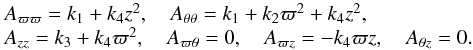 (A.1)Its determinant is
  where k1,k3 are time dependent, positive functions, and k2,k4 non negative constants11.
Similarly, the mean velocity v is obtained from Eqs. (1) and (2). Its components are 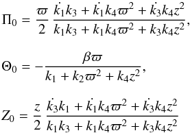 (A.2)with β constant. The dots mean time derivatives. Therefore, a steady state system is only capable of differential rotation.
In the case k ≡ k1 = k3, we get 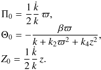 (A.3)
(A.3)
Appendix A.2: Second central moments
The stellar density is obtained with the integration of the phase space density function over the velocity space ΓV, 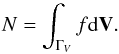 (A.4)For a Schwarzschild velocity distribution,
  , we get
 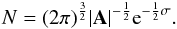 (A.5)Then, the tensor of second central moments, which is defined as
 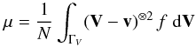 (A.6)satisfies12
 According to Eq. (A.1), its elements have the following functional dependency,
 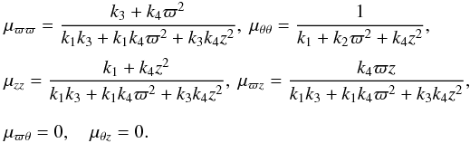 (A.7)The tilt δ of the velocity ellipsoid, ut·μ-1·u = 1, satisfies
 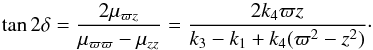 (A.8)In the case k ≡ k1 = k3, the above relationship becomes
 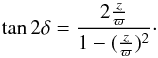 (A.9)Then,
  or
or  , so that one of the principal axes of the velocity ellipsoid points towards the GC.
On the other hand, the vertex deviation ε of the velocity ellipsoid satisfies 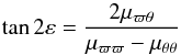 (A.10)so that, if μϖθ = 0, as in the current axisymmetric case, the vertex deviation is null.
Appendix A.3: Moment gradients
The ϖ and z gradients of the central moments are 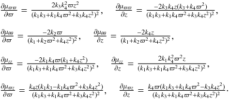 (A.11)Notice that, for z = 0, the values
  , and
, and  are expected to be non-null, in general.
In the GP, the kinematic parameters can be evaluated from the following relationships, 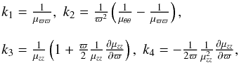 (A.12)which, on the other side, provide the conditions μϖϖ > μθθ,
  , and
, and  .
.
Appendix B: The meaning of U2(0) in the quasi-stationary potential
For a quasi-stationary potential, either in the form of Eq. (31) or in its separable form of Eq. (33), the motion of a star near the GP can be studied by using the reference frame of a circular motion point in the plane. The second equation of motion (e.g., Book I, p. 152) provides the axial component of the angular momentum integral  , while the first equation of motion allows for the description of the radial motion in terms of the effective potential energy
  , as
, as  . The circular orbit in the GP satisfies
  and corresponds to a local minimum of V(ϖ,0) at a radius ϖc, satisfying
 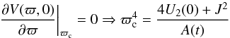 (B.1)under the condition
 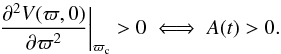 (B.2)Therefore, 4U2(0) + J2 > 0. This is the condition for a stable circular orbit and all the stable non-circular orbits around it. The third equation of motion is consistent with the condition of minimum in z = 0. The circular orbit is a degenerate case of the bounded orbits in its neighbourhood and, from the epicycle approximation, it is possible to prove that they have the same stability as the circular orbit.
In the GP, a repulsive force is associated with a value U2(0) > 0, which allows for stable orbits for all the stars, even for stars with no angular velocity (J = 0), with an oscillating movement along the radial and the vertical directions. This excludes the existence of circular orbits within a radius lower than  . Otherwise, an attractive force is associated with U2(0) < 0, which allows for bounded orbits only for stars trespassing a threshold angular velocity, with a minimum angular momentum integral
  . The other orbits become unstable.
The circular velocity in the plane is given by 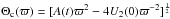 . For low values of ϖ, if U2(0) < 0, Θc(ϖ) decreases similarly to ϖ-1, while if U2(0) > 0, Θc(ϖ) is null for ϖ < ϖmin and increases for ϖ ≥ ϖmin.
Appendix C: Second moments of a n-population mixture
In Cubarsi (1992), Cubarsi & Alcobé (2004), and Pasetto et al. (2012a, 2012b), the velocity moments and cumulants of a two-component mixture were evaluated in terms of the partial statistics and the mean velocity differences between populations. In this appendix, this relationships are generalised to a n-population mixture, by obtaining the total mixture of the second moments in terms of the one-to-one mean velocity differences.
For the ith population, for fixed time and position, let fi represent the velocity distribution function. According to Eq. (A.4), its stellar density is given by  . Each normalised velocity distribution function ψi = fi/Ni defines the respective mean velocity as
  . If the total mixture is written without a subindex and the population fractions are defined as ni = Ni/N, we may obtain the following basic relationships for the normalised density functions, the population fractions, and the mean velocities:
 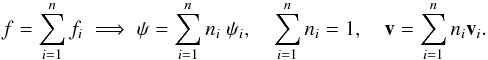 (C.1)The tensor of the second central moments μ, defined in Eq. (A.6), can be expressed working from the population components in terms of the peculiar velocity referred to each population, ui = V − vi, as follows:
 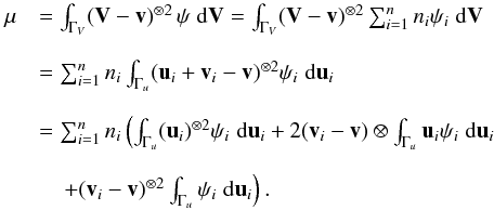 (C.2)Since
  and
and  , by substitution of the mean velocity given in Eq. (C.1), we get
 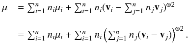 (C.3)We prove the following equality
 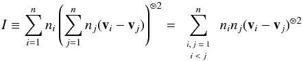 (C.4)by writing I as the addition of the series I1 + I2, so that
 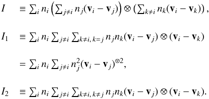 (C.5)The series I1 may be written as13
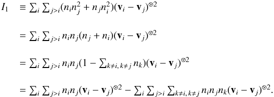 (C.6)Similarly, the series I2 may be written as
 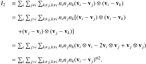 (C.7)
(C.7)
Finally, by addition of Eqs. (C.6) and (C.7) we are led to Eq. (C.4). Then, Eq. (C.3) becomes 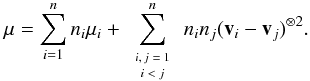 (C.8)Notice, however, that the set of
  differences { (vi − vj) } i,j for i < j are linearly dependent. A reduced set of n − 1 independent quantities is, e.g., { (vk − v1) } k for k > 1, since any difference vi − vj can be obtained as (vi − v1) − (vj − v1).
© ESO, 2014
Current usage metrics show cumulative count of Article Views (full-text article views including HTML views, PDF and ePub downloads, according to the available data) and Abstracts Views on Vision4Press platform.
Data correspond to usage on the plateform after 2015. The current usage metrics is available 48-96 hours after online publication and is updated daily on week days.
Initial download of the metrics may take a while.