| Issue |
A&A
Volume 561, January 2014
|
|
|---|---|---|
| Article Number | A141 | |
| Number of page(s) | 16 | |
| Section | Galactic structure, stellar clusters and populations | |
| DOI | https://doi.org/10.1051/0004-6361/201322436 | |
| Published online | 28 January 2014 | |
Conditions of consistency for multicomponent axisymmetric stellar systems ⋆
Is an axisymmetric model suitable yet?
Dept. Matemàtica Aplicada IV, Universitat Politècnica de Catalunya, 08034 Barcelona, Spain
e-mail: rcubarsi@ma4.upc.edu
Received: 2 August 2013
Accepted: 2 December 2013
Solving the Boltzmann collisionless equation under the axisymmetric hypothesis introduces serious limitations on describing the kinematics of a single stellar system according to the local Galactic observables. Instead of relaxing the hypothesis of axisymmetry, one alternative is to assume a mixture model. For a finite mixture of ellipsoidal velocity distributions, the coexistence of several stellar populations sharing a common potential introduces a set of conditions of consistency that may also constrain the population kinematics. For only a few potentials, the populations may have independent mean velocities and unconstrained velocity ellipsoids. In this paper, we determine which axisymmetric potentials are connected with a more flexible superposition of the stellar populations. The conditions of consistency are checked against recent results derived from kinematic surveys of the solar neighbourhood that include RAdial Velocity Experiment (RAVE) data. Several key observables are used to determine whether the axisymmetric mixture model is able to account for the main features of the local velocity distribution, such as the vertex deviation associated with the second central moment μϖθ, the population radial mean velocities, the radial gradient of the moment μϖz, the tilt of the velocity ellipsoids, and the existence of stars with no net rotation. In addition, the mixture moments for an arbitrary number of populations are derived in terms of the one-to-one mean velocity differences in order to study whether a more populated mixture could add any new features to the velocity distribution that remain unnoticed in a two-component mixture. According to this analysis, the quasi-stationary potential is the only potential allowing arbitrary directions of the population mean velocities. Then, the apparent vertex deviation of the total velocity distribution is due to the difference of the mean velocities of the populations whose velocity ellipsoids have no vertex deviation. For a non-separable potential, the population velocity ellipsoids have the same orientation and point towards the Galactic centre. For a potential separable in addition in cylindrical coordinates, the population velocity ellipsoids may have arbitrary tilt.
Key words: galaxies: kinematics and dynamics / solar neighborhood / galaxies: statistics
Appendices are available in electronic form at http://www.aanda.org
© ESO, 2014
1. Introduction
One of the classical approaches to describing the local kinematics and dynamics of the Galaxy consists of solving the Boltzmann collisionless equation (BCE) by assuming a phase space density function that depends on a quadratic integral of motion whose coefficients are functions of time and position (Chandrasekhar 1960). This involves a number of linear combinations of the classical integrals of the galactic dynamics (Sala 1990). Usually, to simplify the process, a velocity distribution of Schwarzschild type may be assumed, that is, a trivariate Gaussian function in peculiar velocities, which is the maximum entropy distribution with known means and covariances. In this way, the coefficients of the integral of motion are directly related to the mean and the central moments of the velocity distribution. The kinematics of the stellar system is then studied from a statistical viewpoint: the individual orbits of the stars are replaced by the average orbit of their centroid with its associated distribution statistics.
Some symmetries are usually introduced for the mass and velocity distributions to simplify the solution of the BCE. Commonly, it is assumed that the Galaxy is axisymmetric, has a plane of symmetry, and is in a steady state. These hypotheses, however, provide serious limitations to the stellar kinematics, such that it is impossible to describe the local velocity distribution in a realistic way. Following are examples of these well-known limitations. The steady state hypothesis, which yields an axisymmetric potential (Chandrasekhar 1960), supports only stellar systems with differential motion in rotation. A quadratic integral provides a symmetric velocity distribution that cannot account for odd-order central velocity moments (Cubarsi 1992). A quadratic axially symmetric velocity distribution is not able to show any vertex deviation of the velocity ellipsoid (Sala 1990).
In this context, there are basically two complementary alternatives for allow a more flexible description of the stellar kinematics. One is to to relax some of these hypotheses, in particular the one of axial symmetry. The other alternative is to introduce a mixture model associated with several kinematic populations. This paper will explore the latter option, by trying to find out whether it is possible to fit the actual kinematic observables of the Galaxy working from a finite mixture distribution and still maintain the axisymmetric assumption.
From Kapteyn’s theory of the two star streams in 1905, which is to my knowledge the first mixture model in astronomy, there have been different approaches to construct velocity distributions that fit specific observables of the Galaxy. The first statistical and numerical approaches were developed by Kapteyn (1922), Strömberg (1925), and Charlier (1926), in order to fit up to the fourth moments of the velocity distribution. Most kinematical models construct the velocity distribution from a function depending on two or three integrals of motion, and by addition or products of these functions. Quadratic distributions and mixtures of them are a particular case of this. References to these methods can be found in Cubarsi (2010), who describes a mathematical technique that combines the moments method and a maximum entropy distribution function, which is able to fit any desired set of velocity moments of a stellar sample. On the other hand, more recent dynamical models use parametrised velocity distributions that are analytic functions of the action integrals of motion (Binney 2010, 2012; Binney & McMillan 2011), which also allow the constraint of the parameters of the Galactic potential (Ting et al. 2013).
The approach this work revisits benefits from both kinematic and dynamic models. When the quadratic integral of motion is introduced into the BCE, a direct analytical relationship between the potential and the velocity distribution function of each stellar population emerges. On the other hand, if each stellar population is associated with a Gaussian distribution, the segregation of the populations composing the mixture may be worked out from a number of standard statistical and numerical techniques that are independent from the dynamical model.
1.1. Mixture of stellar populations
From a statistical viewpoint, the mixture assumption is a powerful approach, since a well-mixed stellar sample resulting from a single quadratic velocity distribution is actually never found in kinematic surveys. For our stellar mixture, it suffices that the sample can be approximated by a finite number of quadratic distributions. In particular, Schwarzschild distributions may be used instead of other less meaningful quadratic distributions, perhaps at the expense of increasing the number of populations slightly. Then, the whole velocity distribution will show non-vanishing odd-order central moments on condition that the radial and vertical mean velocities of the population components are non-null. Therefore, the introduction of the mixture hypothesis is necessary to gain degrees of freedom for the velocity distribution, although for axially symmetric systems it requires the removal of the steady state hypothesis.
The mixture hypothesis is in agreement with the actual description of the Galaxy through stellar populations conforming its structural components, such as the stellar disc, the stellar halo, the central bulge, or the dark matter halo (e.g., Freeman & Bland-Hawthorn 2002). The local Galactic components are generally fitted from a trivariate Gaussian distribution, although, as will be discussed below, an accurate description of the thin disc may need several Gaussian components.
Recently, Pasetto et al. (2012a, 2012b) adapted the approach based on the cumulants method proposed by Cubarsi (1992) and Cubarsi & Alcobé (2004) to the newest radial velocity data from the RAdial Velocity Experiment (RAVE) survey (Siebert et al. 2011; Zwitter et al. 2008; Steinmetz et al. 2006) for obtaining the kinematics of the thin and thick discs in the solar neighbourhood. They provided the mean velocities and the whole set and trends of the second central moments. Similarly, Moni Bidin et al. (2012) and Casetti-Dinescu et al. (2011) provided moments and gradients for the thick disc, and Carollo et al. (2010) and Smith et al. (2009a, 2009b) discussed the halo kinematics. Also, using the Hipparcos (ESA 1997) and the Geneva-Copenhagen Survey (GCS) catalogues (Nordtröm et al. 2004; Holmberg et al. 2007), Cubarsi et al. (2010) and Alcobé & Cubarsi (2005) provided a kinematic classification of the populations that compose the solar neighbourhood. In addition, smaller Galactic structures produced by a large enough number of stars, such as those of early-type, younger, and older disc stars within the thin disc, were described through more detailed Gaussian multicomponent mixtures (e.g., Bovy et al. 2009; Famaey et al. 2007; Soubiran & Girard 2005).
In most of these cases, the techniques to disentangle the mixture distribution yielded a characterisation of the population components that was totally independent from dynamical assumptions. For example, Pasetto et al. (2012a, 2012b) based their segregation algorithm on previous works involving developments of the moments method in three dimensional velocity space to obtain the best fit for the total distribution cumulants, which are better statistics than the moments. This approach takes advantage of the symmetry shown by the distribution cumulants about the axis along the centroids of a two-component quadratic mixture distribution (Cubarsi 1992). In the beginning, when this method was applied to Hipparcos’s samples (Cubarsi & Alcobé 2004), it was only capable of disentangle two populations. Further improvements, however, based on the construction of a series of nested subsamples depending on optimal properties of a sampling parameter associated with an isolating integral of motion, allowed for identification of several stellar populations contained in the total sample. These included early-type and young disc stars within the thin disc, as well as thin disc, thick disc, and halo populations (Alcobé & Cubarsi 2005). In particular, the segregation of populations improved when the GCS catalogue was used. These populations were associated with partitions of the total sample providing the best estimates for population kinematical parameters and mixture proportions, according to both criteria of minimum chi squared error and maximum partition entropy (Cubarsi et al. 2010).
After segregation, the population kinematics, described through the population means and the second central moments (or covariance matrix), needs to be interpreted in the framework of a dynamical model to test the consistency of these observables with the hypotheses and variables of the model. Most recent results show, among other features, that the disc populations have non-vanishing vertex deviation, the thick disc has a radial mean motion differing from the thin disc, and the halo velocity ellipsoid is slightly tilted.
For a dynamical model to explain such a features, Pasetto et al. (2012b) and Steinmetz (2012) suggest that the axisymmetry assumption should be relaxed, perhaps towards a model with rotational symmetry of 180°. Since these results provide enough material to review in detail the dynamical model sustaining such a mixture of stellar populations in the solar neighbourhood, we shall try to answer that question by testing the consistency of the axisymmetry assumption against the kinematic observables. Often, the validation of the axial symmetry hypothesis is made by identifying the stellar system with a single population, and it ignores the fact that a mixture of populations with arbitrary mean velocities gives a totally different shape to the velocity distribution through their moments and gradients.
1.2. Dynamical model
From a dynamical viewpoint, stellar mixtures can be introduced for the sake of the superposition principle, since the BCE is linear and homogeneous in regard to the phase space density function, for a given potential. Thus, we may assume that the whole stellar system is composed of a finite number of stellar populations in statistical equilibrium, which have the most probable phase distribution of Schwarzschild type (e.g., Ogorodnikov 1965; Lynden-Bell 1967).
The term statistical equilibrium is a notion coming from statistical dynamics that, in analytical dynamics, should be interpreted as associated with an invariant density function in the phase space under the BCE. Dissipative forces, such as dynamical friction, which are essential to statistical dynamics, emerge as solutions of the BCE via non-steady state phase density functions and potentials. Then, for a given potential, the Jeans’ direct problem yields the most probable distribution function for an equilibrium configuration of the Galaxy, and provides us with information about the functional form of the distribution function and the conserved quantities of the stellar motion. Otherwise, when there is some kinematic knowledge about the stars’ integrals of motion, or the velocity distribution function is already known, the Jeans’ inverse problem leads to the most probable potential function.
For a mixture model, the natural approach is the Jeans’ inverse problem, once the populations have been characterised from their velocity distributions. In wide regions of the Galaxy, this is usually done by associating each stellar component with a Schwarzschild distribution function. It is assumed that each population has a centroid that moves with a mean velocity that is a continuous and differentiable function of time and position. This is known as the differential motion of the stellar system and it is guaranteed by the existence of a helicoidal symmetry axis (Chandrasekhar 1939). For that reason, it is generally assumed that the stellar system has rotational symmetry, also referred as axisymmetry. This hypothesis substantially simplifies the dynamical model, although other symmetries, such as point-to-point axial symmetry, could be more appropriate in describing ellipsoidal or spiral mass distributions.
The velocity distribution function should be a time dependent function to react to changes of internal gravitational forces and to allow arbitrary mean velocities of the populations. That is, the mean motion of the populations should not be restricted to rotation alone as is the in case stationary systems.
For the potential, it is assumed that the whole set of populations produces a total self-gravitating system yielding a unique galactic potential, so that the self-gravitation of a single population is negligible. Similar to the velocity distribution function, the potential is expected to be non-stationary.
Then, the BCE relates the dynamics of each stellar population to the common potential shared by all of the population components. When solving the BCE for each population, a set of integrability conditions arises to obtain an admissible potential consistent with all the populations. They will be referred to as conditions of consistency for a multicomponent stellar system. These conditions may force the potential function to adopt a specific functional form, by allowing the velocity and mass1 distributions a number of degrees of freedom.
For axisymmetric systems, these conditions were studied by Cubarsi (1990). It was shown that the more general solution for the potential provides populations differing only in mean rotation. However, particular families of potentials, which are independent of specific population parameters, give rise to kinematically independent populations. This means that the populations may have arbitrary mean velocities and unconstrained velocity ellipsoids. In this case, the centroids of the stellar populations that occupy the same position in the Galaxy do not follow a circular orbit around the symmetry axis. Instead, they may visit other centroid orbits and mix with other populations of their neighbourhood, which is a more realistic situation. Some aspects of the former study can now be reformulated and improved.
In general, there is a tug of war between the potential function and the population velocity ellipsoids in that when the potential function is more general, the stellar populations are more kinematically constrained. This conjures up the well-known Bob Dylan song, “You’re gonna have to serve somebody”.
The aim of this work is to revisit and study in more detail the conditions of consistency for mixtures of axisymmetric systems by determining what potentials are connected with more flexible superposition cases in regard to the population kinematics. It will be tested against actual values of moments and gradients for the thin disc, the thick disc, and the halo, to determine whether an axisymmetric dynamical model is still able to describe the main kinematical features of the solar neighbourhood.
Hereafter, the sections are organised as follows. First, we go over the dynamical model sustaining one stellar population. Second, we study the constraints induced by a finite mixture of populations to the potential and the population velocity distributions. This is organised into several cases, going from greater to less general potential. Third, the observables of the velocity distribution for thin disc, thick disc, and halo samples are checked according to previous cases. In the end, the results are summarised.
2. Chandrasekhar’s approach
In a seminal work2, Chandrasekhar (1960, hereafter Book I) adopted the Jeans’ inverse problem approach for a generalised Schwarzschild velocity distribution. He assumed the phase space density function depending on an integral of motion quadratic in the peculiar velocities and left free the functional dependency on time and space. Such a quadratic integral is the simplest way of labelling one statistical population through the whole set of first and second moments. However, the symmetry of this velocity distribution does not allow non-null odd-order central moments, which means that a mixture of populations is needed to account for other statistics of the distribution. Under particular symmetry hypotheses, basically for an axisymmetric velocity distribution of a disc, Chandrasekhar showed how a common potential shared by two stellar populations introduces links between their kinematic parameters (Book I, p. 126).
This approach is not likely to be valid for the entire Galaxy, but it is a good approximation for the populations existing in solar neighbourhood. Although the population velocity ellipsoids and their rotation curves have a local meaning, we may use the mixture model as a collage representation of the Galaxy. Nevertheless, some properties and symmetries of the velocity distribution and, in particular, the potential should be valid for the entire Galaxy.
For the whole three dimensional space, under the axial symmetry hypothesis, Sala (1990, hereafter Paper I) determined the family of potential functions that was consistent with a quadratic integral of motion, and Cubarsi (1990, hereafter Paper II) studied what constraints would apply to a mixture of stellar populations. However, in 1990 the lag of accuracy in the stellar catalogues, especially in the radial velocity data, left open a long list of suitable models to explain the local kinematics, which now is possible to discuss in more detail.
2.1. Single population
A single stellar population is associated with a quadratic velocity distribution function in the peculiar velocities (u1,u2,u3). The phase space density function is written as f(Q + σ(t,r)) with Q = ∑ i,jAij(t,r) uiuj, where Aij are the elements of a symmetric, positive definite matrix. Hence, Q + σ is an isolating integral of the star’s motion, which is a combination of some of the classical integrals. Generally, from statistical criteria, the velocity distribution is assumed of Schwarzschild type,  , that is, a trivariate Gaussian function in the peculiar velocities. Then, the elements of the covariance matrix are
  , and the equation Q = 1 defines the velocity ellipsoid. From a Bayesian criterion, this is the less informative distribution with known means and covariances.
By substitution of the quadratic density function in the BCE, Chandrasekhar obtained a system of partial differential equations for the potential function U, the scalar function σ, the mean velocity v, namely velocity of the centroid, and the tensor A. These equations are equivalent to the infinite hierarchy of the stellar hydrodynamic equations, which can be reduced to equations of orders n = 0,1,2,3, for the sake of a set of closure conditions (Cubarsi 2007, 2010a).
Under axial symmetry, we also assume z = 0 as a symmetry plane for the mass and the velocity distributions. We note the star’s position r = (ϖ,θ,z) and the velocity V = (Π,Θ,Z).
The BCE may be solved in two blocks. The first one, using the same notation as in Cubarsi (2007, 2013), may be described as 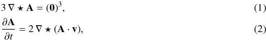 which yields (Paper I) the functional form for the elements of A and the population mean velocity v. They are explicitly written in Appendix A.
The second block, which generalises Chandrasekhar’s equations (Book I, Eq. (3.703)), with the same previous notation may be described as 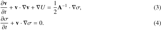 They provide the solution for the potential U and the function σ. These equations are not exactly written as derived by Chandrasekhar. They become equivalent if the new variables Δ = A·v and
  are used. Then we have
 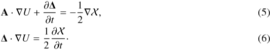 With the elimination of
  between Eqs. (5) and (6), with the new variables
  and
and  , which are appropriate to the symmetry plane of the system, the following set of three second-order partial differential equations for the potential are obtained:
 ![\begin{eqnarray} \begin{array}{r}\displaystyle 2 k_4\left[\tau \frac{\partial^2 U}{\partial\tau^2 } +2 \frac{\partial U}{\partial \tau}-\zeta \frac{\partial^2 U}{\partial \zeta^2 }-2 \frac{\partial U}{\partial \zeta}- (\tau-\zeta) \frac{\partial^2 U}{\partial \tau \partial \zeta}\right] \\~\\\displaystyle +(k_1-k_3) \frac{\partial^2 U}{\partial \tau \partial \zeta}=0, \end{array} \label{chandra1} \\ \begin{array}{l}\displaystyle 2 k_4 \zeta \frac{\partial}{\partial t}\left( \frac{\partial U}{\partial \tau}-\frac{\partial U}{\partial \zeta} \right) \\~\\ \displaystyle + \dot{k_1} \tau \frac{\partial^2 U}{\partial \tau^2}+ k_1 \frac{\partial^2 U}{\partial t \partial \tau} + 2 \dot{k_1} \frac{\partial U}{\partial \tau} +\frac12 \dddot{k_1} + \dot{k_3} \zeta \frac{\partial^2 U}{\partial \tau \partial \zeta}=0, \end{array} \label{chandra2} \\ \begin{array}{l}\displaystyle 2 k_4 \tau \frac{\partial}{\partial t}\left( \frac{\partial U}{\partial \zeta}-\frac{\partial U}{\partial \tau} \right) \\~\\ \displaystyle + \dot{k_3} \zeta \frac{\partial^2 U}{\partial \zeta^2}+ k_3 \frac{\partial^2 U}{\partial t \partial \zeta} + 2 \dot{k_3} \frac{\partial U}{\partial \zeta} +\frac12 \dddot{k_3} + \dot{k_1} \tau \frac{\partial^2 U}{\partial \zeta \partial \tau}=0. \end{array} \label{chandra3} \end{eqnarray}](/articles/aa/full_html/2014/01/aa22436-13/aa22436-13-eq28.png) The particular case k4 → 0 corresponds to Chandrasekhar’s equations for a flat velocity distribution of a rotating disc. This yields the potentials shown in Table 1, Eqs. (I), (II), and (III). Then, the elements of A and the tensor of the second central moments μ do not depend on z. In particular, the moments μϖϖ and μzz do not depend on ϖ and z (which is obvious from the Appendix A.2, by taking k4 = 0). Thus, the velocity distribution is isothermal in these directions3. In addition, if k1 = k3, the distribution is isotropic in the ϖ and z directions.
The particular case k4 → 0 corresponds to Chandrasekhar’s equations for a flat velocity distribution of a rotating disc. This yields the potentials shown in Table 1, Eqs. (I), (II), and (III). Then, the elements of A and the tensor of the second central moments μ do not depend on z. In particular, the moments μϖϖ and μzz do not depend on ϖ and z (which is obvious from the Appendix A.2, by taking k4 = 0). Thus, the velocity distribution is isothermal in these directions3. In addition, if k1 = k3, the distribution is isotropic in the ϖ and z directions.
Potentials that are consistent with a flat velocity distribution.
Some kinematic observables of the Galaxy are analytically related to the potential cases arising from the conditions of consistency for mixtures.
Alternatively, for k4 ≠ 0 the foregoing equations describe a non isothermal three-dimensional distribution and provide two families of compatible potentials. One family of potentials not dependent on the constant k4 are displayed in Table 1, Eqs. (IV) and (V), corresponding to Eq. (2.7) of Paper I. Another family of potentials are dependent on that constant, which are given by Eq. (2.9) of Paper I, are not displayed in Table 1. The latter is a family of Stäckel potentials, separable in prolate ellipsoidal coordinates.
For k4 ≠ 0, the velocity distribution is in general non-isothermal regardless of the solution for the potential. The ϖ and z gradients of the moments μϖϖ and μzz are in general non-null out of the Galactic plane (GP). The velocity ellipsoid of an axially symmetric population has no vertex deviation4, which is associated with the central moment μϖθ.
3. Conditions of consistency for mixtures
Chandrasekhar calls the circumstances under which we can regard a stellar system as consisting of two or more independent populations sharing the same potential conditions of consistency. Since the potential may depend on the population parameters involved in the velocity distribution function, the less the potential depends on them, the less constrained the populations are. In particular, we are interested in potentials allowing the populations to have different mean velocities and arbitrary orientations of the velocity ellipsoids.
For a stellar mixture, say two populations with fractions n′ and n″, the total moment μϖθ depends on the radial and rotational mean velocity differences, according to (Cubarsi 1992),  (10)In addition, according to Appendix A.2, for axisymmetric distributions the partial moments
  and μ″ϖθ vanish. Therefore, if the radial and rotational mean velocity differences between both populations are non-null, the total moment μϖθ is non-null too. Since steady state systems are only capable of rotational differential motion, it is necessary to assume a mixture of time dependent systems.
Depending on the potential function, the axisymmetric mixture model will lead to the following main cases. First, the general case of a potential depending on the constant k4, hereafter referred as axisymmetric general case. Second, the case of a potential that does not depend on k4, hereafter referred to as consistent with a flat velocity distribution, which leads to three particular situations: (a) a potential non-separable in cylindrical coordinates5 with k ≡ k1 = k3, whose time dependency is explicitly expressed in terms of the population parameter k(t); (b) a non-separable potential with k ≡ k1 = k3, referred to as quasi-stationary potential, whose time dependency is carried through a unique function A(t), allowing different mean velocities of the stellar populations, with untilted velocity ellipsoids; and (c) a separable potential satisfying  , with k1 ≠ k3, also depending on time through A(t), allowing arbitrary mean velocities of the populations and arbitrary tilt of the velocity ellipsoids. Both main cases and their subcases are analysed in the the following subsections, by ending with the Table 2 that summarises them.
3.1. Axisymmetric general case
For a single population, the elements of A (Appendix A.1) depend on the functions of time k1(t),k3(t), and on the constants k2,k4,β. However, the constants β and k2 do not appear in Eqs. (7)–(9). There is a trivial case where the same potential is valid for all populations. It happens when the potential depends on the population parameters k1,k3, and k4, but these parameters are proportional among populations, so that we get a system of equations identically planned for each population (Paper II). Then, for a two-component mixture, the constant ratio between parameters is transferred to the second central moments (Appendix A.2), so that they satisfy 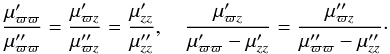 (11)Then, the velocity ellipsoids, in addition to having two proportional semiaxes, have the same orientation in any ϖz plane, that is, the same tilt. The mean velocity components satisfy
  and
and  . Hence, according to Eq. (10), the radial differential motion of the centroids is null and it is impossible to get a non-vanishing total central moment μϖθ.
On the other hand, since the rotation mean velocity Θ0 and the second moment μθθ depend on the constants β and k2, these two quantities are not constrained by the potential. They are independent among populations. Thus, the axisymmetric assumption allows for the potential not to constraint the velocity distribution in the rotation direction.
Such kinematical behaviour is not far from the actual portrait of the Galaxy in the solar neighbourhood; although, as is well known, small violations of this ideal situation have long since been observed, such as the vertex deviation, mainly for the thin disc, and the existence of non-null central moments involving odd powers of the radial velocity (Erickson 1975).
3.2. Flat velocity distribution
The solution for a potential that does not depend on k4 (but depends on k1,k3) is the same as the potential obtained with k4 = 0, although the populations are still k4-dependent. This is a generalisation of the case studied in Book I (pp. 116–121), associated with an ideal rotating disc. An isothermal velocity distribution in the direction perpendicular to the disc does not imply an isothermal mass distribution, but a relatively small scale height, since the dependence of the mass distribution on z comes through the potential as well6.
The general solution for the potential will not depend on k4 when the terms being multiplied by this constant in the Eqs. (7)−(9) are zero7. This provides two additional and fundamental integrability conditions ![\begin{eqnarray} \label{conditions1} &&\tau \frac{\partial^2 U}{\partial\tau^2 }+2 \frac{\partial U}{\partial \tau}-\zeta \frac{\partial^2 U}{\partial \zeta^2 }-2 \frac{\partial U}{\partial \zeta}- (\tau-\zeta) \frac{\partial^2 U}{\partial \tau \partial \zeta}=0, \\[2mm]\label{conditions2} && \frac{\partial}{\partial t}\left( \frac{\partial U}{\partial \tau}-\frac{\partial U}{\partial \zeta} \right)=0. \end{eqnarray}](/articles/aa/full_html/2014/01/aa22436-13/aa22436-13-eq83.png) The condition of Eq. (12) leads to a potential function in the form
The condition of Eq. (12) leads to a potential function in the form 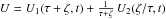 (a deduction can be found in Paper II, Appendix C). The condition of Eq. (13) forces U2 to be time-independent. Then, Eq. (7) simply remains as
 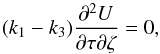 (14)and Eqs. (8) and (9) become
 ![\begin{equation} \begin{array}{l} \displaystyle \dot{k_1} \tau \frac{\partial^2 U}{\partial \tau^2}+ k_1 \frac{\partial^2 U}{\partial t \partial \tau} + 2 \dot{k_1} \frac{\partial U}{\partial \tau} +\frac12 \dddot{k_1} + \dot{k_3} \zeta \frac{\partial^2 U}{\partial \tau \partial \zeta}=0,\\[4mm] \displaystyle \dot{k_3} \zeta \frac{\partial^2 U}{\partial \zeta^2}+ k_3 \frac{\partial^2 U}{\partial t \partial \zeta} + 2 \dot{k_3} \frac{\partial U}{\partial \zeta} +\frac12 \dddot{k_3} + \dot{k_1} \tau \frac{\partial^2 U}{\partial \zeta \partial \tau}=0. \label{chandra-remain} \end{array} \end{equation}](/articles/aa/full_html/2014/01/aa22436-13/aa22436-13-eq87.png) (15)The conditions of consistency now have to be studied in relation to Eq. (14). We investigate the cases where
(15)The conditions of consistency now have to be studied in relation to Eq. (14). We investigate the cases where  is null or non-null separately. These correspond to a non-separable or separable potential in cylindrical coordinates, respectively8.
For the particular case of a steady state system, where k1 and k3 are constant, and  , both relationships in Eq. (15) vanish. We then obtain the stationary potential
 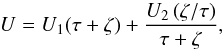 (16)which is independent from the population parameters. A steady state system is thus free from conditions of consistency, but only allows differential rotation of populations since
  , as is obvious from Eq. (A.2). The overall vertex deviation of the mixture distribution is null and the most significant odd-order central moments are forbidden.
3.2.1. Non-separable potential
According to Eq. (14), if  then k ≡ k1 = k3. The condition is directly related to the tilt of the velocity ellipsoid. In a three-dimensional velocity distribution with k4 ≠ 0, according to Eq. (A.9), if k1 = k3, one of the principal axes of the velocity ellipsoid points towards the Galactic centre (GC). Then, the population velocity ellipsoids are not tilted.
In this case, the existence of a quadratic integral involves three independent integrals of motion (Paper I) and allows for a general solution for the potential in the following form: 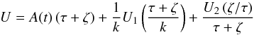 (17)with the function A(t) satisfying
  (18)We may assume that the two possible terms of U1, which are proportional to
  and
and  are already accounted for in the first and third terms of Eq. (17), respectively.
The above potential, if expressed in spherical coordinates (R,θ,φ), with R2 = r2 + z2 and tanφ = z/r, satisfies the property  (19)that is, R2U(R,φ) is separable in addition in spherical coordinates.
The first term of Eq. (17) is an harmonic potential. For a stellar mixture, A(t) must be the same computed from either populations, and determines the function k(t) according to a linear differential equation. Thus, if we eliminate the constant c in Eq. (18), by multiplying by k2 and taking the time derivative, we find  (20)For a given A(t), this is a third order homogeneous equation in k(t). If ϕ1(t),ϕ2(t),ϕ3(t) are three linearly independent solutions of Eq. (20), then its general solution is
  (21)Therefore, in each population, k(t) must be a particular solution to the above general solution9.
An attractive force is associated with values A > 0, which guarantees the existence of stable orbits. In particular, if A > 0 is constant, the above differential equation becomes  , so that
  (22)The term U1 in Eq. (17) is a spherical potential associated with a generic central force. In the general case U1 ≠ 0, the potential also depends on time through the function k(t), which is a population parameter.
The term with U2 may depend on the elevation angle about the GP and it is responsible for producing a flattened potential. Similar to Binney & McMillan (2011), we find that non-spherical potentials may coexist with velocity distributions with a vanishing tilt of the velocity ellipsoid. Notice that  is of the same type as the perturbation of a point-mass potential induced by a tidal force, although as we assumed a symmetry plane, this force is symmetric about this plane. Hence, this force can only have the direction perpendicular to the GP or a direction along the same plane, with the application point in the GC. The interest of a potential sufficiently general like Eq. (17) is that its functional dependence may support its own perturbations.
According to Appendix A.1, the non-rotational mean motion of a population is associated with time variations of the stellar system. In the current case, these velocity components satisfy  (23)meaning that each population centroid moves on a circular conic surface with the apex in the GC. For a mixture of two populations, the second central moments satisfy
 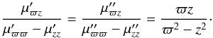 (24)Then, the semiaxes of the velocity ellipsoids are not proportional as in the general case, but have vanishing tilt.
Nevertheless, as remarked above, the spherical potential term  must be common among the populations. Then, for a two population mixture, it is easily deduced that k′ and k″ must be proportional. Therefore, according to Eq. (23), the mean velocity differences satisfy
 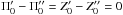 .
.
More precisely, being k′ and k″ solutions of the same linear and homogeneous differential equation Eq. (20), k′ is proportional to k″ if, and only if,  . Hence, if, and only if, k′ and k″ are linearly dependent. For that reason, for a potential to allow different non-rotational motion of the centroids, we have to search for a particular solution to Eq. (17) that is independent from the quantity
  .
.
Therefore, a potential containing a general spherical term does not allow independent radial and vertical mean motions of the populations.
3.2.2. Quasi-stationary potential
For k ≡ k1 = k3, in regard to Eqs. (12) and (13), we define 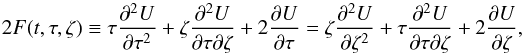 (25)
(25) (26)
Then, both expressions in Eq. (15) can be written as a unique equation
(26)
Then, both expressions in Eq. (15) can be written as a unique equation  (27)By Eq. (20), since
  , Eq. (27) then becomes
  (28)As the functions A(t),F(t,τ,ζ), and G(t,τ,ζ) depend on the potential, a potential not dependent on
  , which is population-dependent, must satisfy F = A. Therefore, G = Ȧ is also held. Hence, by Eq. (26), the potential must satisfy
  . Then, by Eq. (17) we find
  (29)By taking Eq. (26) into account, the above condition for a potential allowing for different radial and vertical population mean velocities can also be expressed as
  (30)The time derivative of the potential has to be separable in cylindrical coordinates. We are then left with the potential
 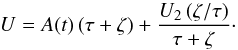 (31)This potential will be referred to as a quasi-stationary potential, since if we force the general potential Eq. (17) to be stationary, we get the same solution as Eq. (31) (with U1 = 0), but with the condition A = constant. Thus, the quasi-stationary potential depends on time through a unique function A(t), which is population independent.
For U2 > 0, the second term of Eq. (31) can be associated with a repulsive force, which is relevant at low distances from the GC. It may be interpreted as a gravitational force due to the outer mass of a dark matter halo, and it is then possible to have stable orbits even for those stars with no net angular velocity (Appendix B). In the GP, this repulsive force would produce a decreasing circular velocity towards the centre. This seems to be the actual situation, mainly for the Galactic components existing in the solar neighbourhood (Reid et al. 2009; Levine et al. 2008; Xue et al. 2008). Otherwise, for U2 < 0, the circular velocity would increase towards the centre, where it would be a non-realistic singularity. However, this model is only valid where the motion of stars admits a quadratic integral in peculiar velocities, so that it might not be extrapolated near the GC.
It is interesting to note the difference between the potential of a steady state system and the stationary potential of a non-stationary system. In steady state systems, k is constant. Then, Chandrasekhar’s equations yield a stationary potential in the form of Eq. (16). Indeed, if we assume  in Eq. (17), we are left with Eq. (16). However, if we force the potential of Eq. (17) to be stationary in a stellar system where k is not constant, which means that A(t) must be constant, we obtain the quasi-stationary potential of Eq. (31), which is a very particlar case of Eq. (16). Therefore, in non-steady state systems, only a particular family of stationary potentials is allowed.
As the functional dependence of k is given by Eq. (21), k(t) has three degrees of freedom for each population10. Hence, this functional dependence allows the mean velocities of each population to be decoupled, 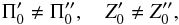 which provides the possibility of an apparent vertex deviation for the total velocity distribution.
However, as Eq. (23) is satisfied, the velocity differences are not totally independent. They still maintain the proportion  (32)that of populations moving on a conic surface with the apex in the GC.
3.2.3. Separable potential
When k1 and k3 are non-equal functions of time, both satisfying Eq. (20), according to Eq. (14), the potential must separable in addition in cylindrical coordinates, that is,  . Then, the potential becomes a particular case of the quasi-stationary potential Eq. (31), with U1 = 0,
  (33)with B and C constant. We may assume C = 0 by continuity conditions in the plane z = 0. This is a first order approximation of the general potential Eq. (17) near the GP.
Both relationships in Eq. (15) allow for a decoupling of kinematics in the directions ϖ and z. This is related to the existence of an extra isolating integral of motion involving the vertical velocity alone (Paper I). However, the decoupling is not absolute like in Chandrasekhar’s case with k4 = 0 (Book I, Eq. (3.743)), since the potential must be consistent with the general solution found in Eq. (17).
According to Appendix A.1, the case k1 ≠ k3 allows for a total independence of the population mean velocities and of the shape of the velocity ellipsoids. According to Eq. (A.8), their tilt may have a non-vanishing tilt. In addition, the overall distribution may show an apparent vertex deviation. This is the only axisymmetric case allowing for a total independence of the population’s kinematics. However, notice that the necessary and sufficient condition for a tilted velocity ellipsoid is k1 ≠ k3, while the separability of the potential is only a necessary condition. A potential may be separable and the ellipsoid may have no tilt if k1 = k3.
If A(t) is constant, that is, if the potential is stationary, the population centroids move, in general, on a toroidal surface with elliptical section (Cubarsi et al. 1990) or, in particular cases, over a cone, a hyperboloid, an ellipsoid, or a circular band restricted to the GP.
The second term of Eq. (33), as a particular case of the quasi-stationary potential, is related to the angular momentum integral of the stars with stable orbits. For disc stars, if B > 0, this term is associated with a repulsive force (Appendix B). It is then possible to have stable orbits even for those stars with no net angular velocity. Otherwise, if B < 0, the potential term is associated with an attractive force that only allows stable orbits for stars trespassing a threshold angular velocity.
In summary, Table 2 shows how some observables are related to the different potential cases arising from the conditions of consistency. The observables are the ratio between semiaxes of the velocity ellipsoids, the difference between radial and vertical mean velocities of the populations, the angles for the vertex deviation ε and the tilt δ of the population velocity ellipsoids, and the sign of the moment μϖz in terms of z (which is discussed below). The quantities without accents refer to the total stellar distribution and those with accents refer to two populations, which are easily generalised to any finite mixture. Each stellar population is assumed of Schwarzschild type, so that the deviation angles with accents apply to real velocity ellipsoids. However, the angles without accents measure the apparent vertex deviation and tilt of the whole stellar distribution from their total second central moments. The main cases for the potential are: an axisymmetric general case, for a potential depending on the population parameter k4, and a flat velocity distribution, for a potential not dependent on the population parameter k4. This case splits into: the non-separable potential (Eq. (17)), when the potential depends on the population parameter k; the quasi-stationary potential (Eq. (31), when the potential does not depend on the population parameter k; and the separable potential (Eq. (33)), when the potential does not depend on the population parameters k1 ≠ k3. Therefore, regarding to the potential, the cases range from general to particular.
Figure 1 displays the stellar density of a single stellar population obtained for the harmonic potential (left); and, in contrast, the stellar density for the quasi-stationary, non-separable potential (centre), which allows for stellar orbits all around the GC; and the stellar density for the separable potential (right), for which the stars orbit around the rotation axis of the stellar system.
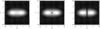 |
Fig. 1 Stellar density of a single population for the harmonic potential (left), for the non-separable quasi-stationary potential (centre), and for the potential separable in addition in cylindrical coordinates (right). |
4. The solar neighbourhood
We shall check the kinematic features of the local thin disc, thick disc, and halo components, in connection to the cases studied above to examine whether the hypothesis of axisymmetry is valid yet. We shall pay attention to the velocity moments and gradients, and, in particular, to four key observables: the vertex deviation, the trend of the moment μϖz around the sun, the tilt of the velocity ellipsoid, and the existence of stars without net rotation.
4.1. Thin disc
The results obtained by Pasetto et al. (2012b) show that the velocity moments μϖϖ and μzz for the thin disc are approximately constant in the solar neighbourhood (z ≈ 0), the latter slightly decreasing towards the Galactic anticentre, with an anisotropy coefficient μzz/μϖϖ ≠ 1, with the same decreasing trend. In addition, the moment μθθ also increases towards the GC. According to the expressions of the moment gradients in Eq. (A.11) (Appendix A.3), by fixing z = 0, we get a constant value for  , while
  and
and  are decreasing functions of ϖ. Therefore, the thin disc, or the stellar populations composing the thin disc, have a velocity distribution which, in good approximation, are consistent with such a trend and with a small value of k4, close to that of a flat velocity distribution, and a small, but non-null value of k2.
The thin disc shows a net vertex deviation and is the Galactic component in the solar neighbourhood more distant from the steady state. According to our analysis, it is possible to account for an apparent vertex deviation, even under axisymmetry, for the sake of the difference of radial and rotation mean velocities. Such a feature is in agreement with a previous analysis (Cubarsi 2010), where the stellar subsystems around whose the kinematics of the thin disc is articulated became undisclosed by working from increasingly eccentricity layers. A maximum entropy method was applied to fit the velocity moments up to the tenth order, without assuming any type of symmetry or any specific velocity distribution other than a single maximum entropy density function. The thin disc stars drawn from the GCS catalogue with very low planar eccentricity could be associated with star streams with a relatively small number of stars. However, as increasing the sample up to eccentricity e = 0.15 (with maximum height zmax = 0.5 pc), the sample of 9545 stars had incorporated and averaged the features of the discrete moving groups, and showed a clear and general trend. Its velocity distribution was close to a mixture of two ellipsoidal components, each one without vertex deviation, but producing an apparent vertex deviation of the whole distribution, as displayed in Fig. 2 (U = −Π is the radial heliocentric velocity, positive towards the GC, and V is the rotational heliocentric velocity, positive in the direction of the Galactic rotation), with approximate dispersions (13,9,11) km s-1 and (14,7,11) km s-1, a difference of mean velocities of (43,26, −22) km s-1, and proportions 80% and 20%, respectively. One component contains the main groups of Hyades and Pleiades, and the other is built around the Sirius and UMa streams. As the eccentricity is continuously increased up to e = 0.30 (11 826 stars), a unimodal velocity distribution, similar to that of the thin disc (Cubarsi et al. 2010), was reached, with dispersions (30,18.5,15.5) km s-1, and with a vertex deviation of about 10°, by orienting the velocity ellipsoid in the direction connecting both previous centroids. Therefore, the thin disc may be approximately fitted from a mixture of two populations with no vertex deviation, with a significant radial mean velocity difference, in addition to an overlapped old disc component, all of them consistent with a mixture of axial symmetric populations. This kinematic interpretation of the vertex deviation is also in agreement with recent studies of the shape of velocity ellipsoids in spiral galaxies (Vorobyov & Theis 2008), confirming that the magnitude of the vertex deviation is not correlated with the gravitational potential, but is strongly correlated with the spatial gradients of the mean stellar velocities.
In contrast to our finite mixture distribution approach, other models prefer to describe the thin disc from a continuous mixture distribution (e.g., Binney 2010, 2012), by integrating the distribution functions associated with different ages and velocity dispersions, as a consequence of a continuous star formation rate. However, it is no doubt concerning that discrete populations exist in the solar neighbourhood, which, in addition, account for most stars of the local samples. It is not a bad approach, then, to handle the continuous mixture of the remaining disc stars through another discrete Gaussian component to apply the current dynamic model for quadratic distributions.
It is more difficult to explain the behaviour of the moment μϖz around the GP, as described by Pasetto et al. (2012b), than it is to explain the vertex deviation. The moment takes opposite signs at different distances from the GC for non-null z values. For instance, by picking up only values with uncertainty below 2σ levels, we see in Table 6 (and also the third column of Fig. 4), in Pasetto et al. (2012b), that stars with height − 0.3 < z ≤ − 0.1 kpc have increasing moment values − 83 ≤ μϖz ≤ 34 km2 s-2, as the distance to the GC increases from 8 to 8.8 kpc. Similarly, for the same range of distances to the GC, stars with height 0.1 < z ≤ 0.3 kpc have decreasing moments 121 ≤ μϖz ≤ − 98 km2 s-2. In both cases, if these values were meaningful, the moment μϖz would take opposite values around the solar position for a fixed height, z ≠ 0. Therefore, according to Eq. (A.8), the apparent tilt of the thin disc distribution oscillates around that of an ellipsoid pointing to the GC. This feature is boosted if the stars belong to the bins z ∈ ( − 0.5, − 0.3] and z ∈ (0.3,0.5], although the error bars are then much greater.
The central moment μϖz, from Eq. (A.7) in the Appendix A.2, is proportional to z by a factor that is always positive. Therefore, we might expect moment values with constant sign on both sides of the GP, positive if z > 0, negative if z < 0, and null on the plane. Then, for a single population, the moment μϖz can never show such an actual trend.
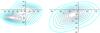 |
Fig. 2 Velocity distribution isocontours projected onto the GP for stars with eccentricity up to 0.15 (left) and up to 0.30 (right), both for GCS stars (Cubarsi 2010). |
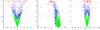 |
Fig. 3 Fraction F of kinetic energy (square root) not involved in rotation as a function of the Galactocentric rotation velocities U,V,W for thin disc (green), thick disc (blue), and halo stars (red). |
To explain this possible behaviour of that moment it is necessary once more to use the mixture approach. For a two-component mixture we obtain, similar to Eq. (10),  (34)now with non-null partial moments, which have the same sign as z. To allow a change of sign in the total moment near the solar position for low values of | z | ≠ 0, it is necessary (1) that the third term involving the mean velocity differences be non-null, and (2) that their sign be opposite to that of the partial moments. This is only possible if
  has the sign of − z.
Thus, in a first instance, the general axisymmetric case and the non-separable potential case of a flat velocity distribution have to be excluded because they provide values  and . On the other hand, the particular case of a quasi-stationary potential with k ≡ k1 = k3 does allow unconstrained mean velocities (
 ) and provides values
  that yield non-null values for
  and
and  . However, we get
 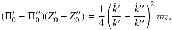 which has the same sign as z. Hence, this case would also have to be excluded, at least for a two-population mixture.
Then, we could still wonder if a mixture of more than two populations with unconstrained mean velocities would be able to provide a contribution of the same sign than − z in the generalisation of Eq. (34). The answer is no. In Appendix C, a general mixture with an arbitrary number of components is studied. It is found that the contribution of the population mean velocity differences to the second moments is of the same type as for a two-component mixture, as shown in Eq. (C.8). Hence, the same reasoning about the sign of that moment is proven to be valid for a general mixture.
If actual data are to be trusted, to explain the trend of this moment in the solar neighbourhood only the case k1 ≠ k3 with a separable potential would be left, where the product may have an arbitrary sign. Therefore, we cannot discard the possibility that such a behaviour is due to a sampling problem, although it could also be due to small local deviations from the non-separable, quasi-stationary potential.
4.2. Thick disc
For the thick disc, Casetti-Dinescu et al. (2011) obtain vanishing values for the moment gradients and , a nearly zero value within the error bars of  , and clearly non-vanishing values of
  , and
, and  . It is easy to verify that these quantities are qualitatively in agreement with the assumption of a single population with k4 ≠ 0, although small. Thus, by naming ϵ ≡ k4, from Appendix A.3 we write explicitly the moment gradients in terms of ϵ and z, for fixed ϖ. We then get the following order estimations:
 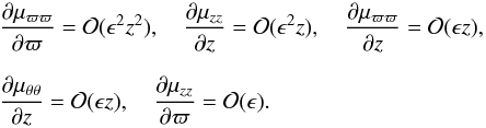 (35)In addition, the value is approximately constant and non-null, unless k2 = 0. Notice that the gradients of moments that are odd in the variable z may show diminished values, since the samples were selected by different values of | z |, by averaging stars from both sides of the symmetry plane. Therefore, the thick disc kinematics may be described from a single quadratic population with small, but non-null values of k4 and k2. Similarly, these authors find a small value for
  , which is also consistent with the small values of k4 and z.
On the other hand, they find a non-vanishing tilt of 8.6° ± 1.8 for the thick disc velocity ellipsoid, which should be associated with the separable potential, while the vertex deviation is consistent with zero. The non-vanishing tilt was also found by Siebert et al. (2008) and Fuchs et al. (2009). The general kinematic features of the thick disc are also in agreement with the results obtained by Carollo et al. (2010), Pasetto et al. (2012a), and Moni Bidin et al. (2012), although the latter find a non-null vertex deviation of thick disc stars, which increases with the distance to the GC. It is worthwhile to remark that an axial symmetric model with a mean velocity non-symmetric about the plane z = 0 provides a vertex deviation proportional to z (Paper II, Appendix A).
In addition, for the thick disc there is evidence of a net peculiar radial mean velocity towards the GC of 9.2 ± 1.1 km s-1, that is, U ≈ 19 km s-1 referred to the Sun. The result, which agrees with those of Girard et al. (2006), Bramich et al. (2008), and Smith et al. (2009b), was also found by Cubarsi & Alcobé (2006) by working from nested Hipparcos subsamples, despite Casetti-Dinescu et al. (2011) saying that Hipparcos-based results are unlikely to detect this. These nested Hipparcos subsamples were built to contain an increasing number of thick disc stars. They showed a trend that was interpreted as a single point-axial symmetric population (Juan-Zornoza 1995) approaching an ideal, axial, steady state population, with no net Galactocentric radial mean velocity. The zero mean velocity of this ideal population was then extrapolated by leading to a heliocentric velocity of ca. 20 km s-1 towards the GC.
Hence, this analysis confirms that a mixture of stellar populations with independent radial differential motions is required to explain the disc kinematics, which is still possible in axially symmetrical systems.
4.3. Halo
Halo stars, either from the inner or the outer halo, despite the uncertainty of their velocity statistics, seem to have velocity ellipsoids with non-vanishing tilt (Carollo et al. 2010; Smith et al. 2009a; Chiba & Beers 2000), and also a differentiated mean radial motion (Smith et al. 2009b), in addition to a retrograde rotation of the outer halo. The outer halo has close values of μϖϖ and μθθ, by providing a nearly zero value of k2, which, according to Eq. (A.2), would correspond to an almost rigid body rotation for fixed values of z. However, a more detailed analysis (Smith et al. 2009a) suggests that the halo, in particular the inner halo, would be approximately at rest, close to steadiness and spherical symmetry, aside from a slight masking produced by some disc and bulge stars. These authors, based on an analysis of integrals of motion and Poisson equation, claim that the potential associated with a triaxial velocity dispersion tensor of the halo should be spherical and the ellipsoid should not show any tilt. However, according to the authors, although the potential of the ellipsoidal dark halo is the one dominant over the whole Galaxy, which is associated with the harmonic potential term, the total potential produced by the mixture of the Galactic components, and in particular by the disc, breaks the overall sphericity.
Our approach is totally different from the approach of Smith et al. (2009a). We consider a time dependent potential and specifically avoid the Poisson equation, which they used as the main reason to reject the term depending on the elevation angle in Eq. (17). Further, we need streaming motions (which they rejected) to account for asymmetries in the disc velocity distribution. However, somehow, we are led to a similar result: a general spherical potential is inconsistent with a tilted velocity ellipsoid. The harmonic potential is the only spherical potential allowing tilted ellipsoids. However, the term depending on the elevation angle in Eq. (31) is not always responsible for the tilt. It only occurs when k1 ≠ k3, by forcing the potential to be separable in cylindrical coordinates.
In order to get unconstrained population mean velocities, once again U1 = 0 is required. That is, the spherical terms of the potential must be proportional to (τ + ζ) and (τ + ζ)-1.
A similar analysis, as in the previous section, of the mean velocity gradients provides an order estimation  , which agrees with non-null, but small values of k4. Thus, each halo component could be fitted through a single Schwarzschild distribution with no vertex deviation.
In addition, according to Appendix B, the existence of stars with null Galactocentric rotation velocity requires a potential with a positive value of U2 in Eq. (31), associated with a repulsive force field. These stars can be drawn, e.g., from a GCS classified sample (Cubarsi et al. 2010). For each star, we compute the fraction 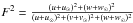 of kinetic energy, which is not involved in the rotation. In Fig. 4.1, the plot F against the Galactocentric velocities U,V,W uses colours to label the stars belonging to the thin disc (green), the thick disc (blue), and the halo (red), as they were segregated in Cubarsi et al. (2010). For the Sun, we assumed a Galactocentric rotation v⊙ = 220 km s-1 and radial and vertical peculiar velocities u⊙ = 10 km s-1 and w⊙ = 7 km s-1, opposite from the heliocentric centroid velocity of the sample. We also assumed that the radial and vertical Galactocentric velocities of the local centroid vanished. The graphs show that there are stars with no net rotation that belongs to the halo, which have a symmetric distribution in the radial and vertical motions. These stars have the highest eccentricities. The shape of the graph is basically the same when a slightly different absolute solar motion is adopted.
5. Conclusions
To simplify the solution of Chandrasekhar’s equations, it is necessary introduce some symmetries for the mass and the velocity distributions, such as the assumptions of axisymmetry, steady state, or Galactic plane of symmetry. These hypotheses provide serious limitations for describing, in a realistic way, the kinematic observables of the Galaxy. Recently, several kinematic analyses using the newest radial velocity data from the RAVE survey confirmed that the thin disc had non-vanishing vertex deviation, the thick disc had a radial mean motion differing from that of the thin disc, and the halo velocity ellipsoid was likely to be tilted. It was suggested (Pasetto et al. 2012b; Steinmetz 2012) that the axisymmetry assumption should be relaxed towards a model with a rotational symmetry of 180° to account for some of these features. In this paper, we have adopted a mixture model to check the axisymmetric hypothesis. We have determined what axisymmetric potentials are connected with a more flexible superposition of stellar populations, so that they can describe, in a realistic way, the main kinematic features of the solar neighbourhood.
The conditions of consistency are integrability conditions allowing a stellar system composed of several independent populations to share the same potential function in the BCE. Since the potential may depend on the population parameters involved in the velocity distribution, the less the potential depends on them, the less kinematically constrained the populations will be. Thus, in solving the BCE, we looked for potentials permitting different mean velocities of the populations and arbitrary orientation of the velocity ellipsoids. We found that these potentials do not depend on the population parameter k4. They were consistent with a flat velocity distribution and did not constrain the axes of the velocity ellipsoids.
For k ≡ k1 = k3, we obtained the family of potentials of Eq. (31), designated as quasi-stationary, which, in general, are non-separable in cylindrical coordinates. Their time dependency is carried through a unique function A(t), which is population independent. Then, the stellar populations have untilted velocity ellipsoids and their centroids move on conic surfaces with the apex in the GC.
The other possible solution was a potential separable in cylindrical coordinates, for which the values k1 and k3 may differ. Their time dependency is also carried through a unique function A(t). If k1 ≠ k3, in addition to unconstrained mean velocities, the populations show an arbitrary tilt of the velocity ellipsoids.
Therefore, with the mixture model, we should be able to fit the general features of the actual velocity distribution in the solar neighbourhood without the requirement of relaxing the axisymmetrical hypothesis. Four key observables have been evaluated to prove it.
First, the vertex deviation, which is clearly non-zero for the thin disc. There is a tendency to associate the vertex deviation of the velocity ellipsoid with the break of axisymmetry, which is only true for a single population. The vertex deviation is easily explained as a result of the superposition of two or more axisymmetric populations with different radial and rotational mean velocities. Such a situation requires the quasi-stationary potential Eq. (31). This interpretation of the vertex deviation was confirmed by the fact that the isocontours of the velocity distribution obtained by Cubarsi (2010) for disc stars with eccentricities lower than 0.15 gave a clear picture of a bimodal distribution, each mode approximately ellipsoidal with no vertex deviation, which were overlaid with a significant difference in the radial mean velocities. Upon completion of the sample with higher eccentricity stars, the overall thin disc distribution arose as a mixture of three axisymmetric populations with an apparent vertex deviation.
The second key observable is the behaviour of the radial gradient of the moment μϖz in the solar neighbourhood. If the results of Pasetto et al. (2012b) are right, although the moment is nearly null at the GP, there is a change of sign of this moment, above and below the plane, near the solar radius, instead of maintaining a constant sign, as a single population would do. To account for this behaviour, it is not sufficient to consider a population mixture with different radial and vertical mean velocities. It is necessary that the differences  and
and  be non-proportional. This is only possible for a quasi-stationary potential with k1 ≠ k3, which yields the potential separable in cylindrical coordinates of Eq. (33).
The possibility of explaining such a behaviour from a mixture of three or more populations with a non-separable potential was also dismissed. The second moments of a mixture with an arbitrary number of populations were obtained with this purpose in the Appendix C. They were related to the one-to-one mean velocity differences to verify that the change of sign of μϖz is only possible under a separable potential, regardless of the number of population components.
The third point to check is about the tilt of the population velocity ellipsoids. The tilt could be non-null for thick disc and halo stars. The most recent analyses show a preference for accepting a slight tilt of both Galactic components. If these results are conclusive, they are consistent with a separable potential with k1 ≠ k3.
The fourth and last key observable is the existence of halo stars with no net rotation. This is consistent with a potential more general than the harmonic one, such as Eq. (17), containing a term U2 > 0 associated with a repulsive force, e.g., due to the outer mass of a dark matter halo.
According to these results, the axisymmetric quasi-stationary potential is consistent with the local Galactic observables. The non-separable potential, with k1 = k3, even containing a term depending on the elevation angle, would be admissible for a mixture of populations with non-tilted ellipsoids. Then, the slight tilt of the halo and the uncertain tilt of the thick disc should be interpreted as local perturbations or a statistical fluctuations, instead of intrinsic characteristics of the stellar system. Otherwise, the potential separable in cylindrical coordinates, with k1 ≠ k3, supports populations with tilted velocity ellipsoids as a general feature.
The analysis undertaken in this paper is obviously limited by its own hypotheses. By taking the validity of the BCE for granted, the two basic assumptions are: first, that a stellar population is associated with a quadratic velocity distribution; and, second, that the whole stellar system is obtained as a finite mixture of populations.
In regards to the first assumption, we may recall that, although the hypothesis fails when a quadratic distribution is associated with a moving group with hundreds of stars, if kinematically unbiased samples of thousands of stars are considered, the velocity distribution generally shows a multimodal shape, close to a superposition of quadratic distributions. Therefore, the first hypothesis should be accepted for describing general trends of large stellar populations, but admitting that local statistical fluctuations may exist depending on the size and bias of the sample.
On the other hand, the limitations concerning the second assumption will depend on the goodness of the fit when a real continuous mixture of stellar populations is replaced by a single quadratic population. In two cases, the error produced by such an approximation is negligible. One case occurs when a continuous mixture represents a small fraction of the total sample, which is composed mostly of discrete populations. Then, the approximation may produce small changes in the wings of the discrete distributions. As mentioned above, this is the case in the solar neighbourhood. The other case involves a continuous mixture of Gaussian distributions with nearly the same mean takes place, by producing a positive excess of kurtosis. In that case, the resulting distribution is also quadratic (Cubarsi 2007) and, therefore, is consistent with the current model.
The current analysis started with an additional assumption to be tested: the axial symmetry. We have concluded that, even under this hypothesis, it is possible to describe the general kinematic features of the solar neighbourhood from a finite mixture of quadratic populations. Although from a statistical viewpoint both basic hypotheses do not introduce serious limitations to our problem, from a dynamical viewpoint it is clear that the solutions for the potential have been greatly reduced. In this regard, two further analyses could be done to find out whether more general potentials are admissible. In the first, we would investigate the conditions of consistency for point-axial symmetry models (Juan-Zornoza 1995; Sanz-Subirana 1987). That is, to relax the axisymmetric hypothesis to see how this affects the potential. In the second analysis, we would relax the assumption of a symmetry plane for the mass and velocity distributions, because, as we said, it is convenient that the general solution for the potential could account for the self perturbations, such as those produced by tidal forces, which may occur out of the symmetry plane, yielding then to potentials and velocity distributions that are non-even functions in the variable z.
Online material
Appendix A: Axisymmetric stellar system
The importance of the axial symmetry hypothesis arises from two of Chandrasekhar’s results (Chandrasekhar 1960, pp. 104−105). One result is that a stellar system in steady state with differential motions is characterised by an axis of helical symmetry. The other result is that if a stellar system is in steady state, the potential is axisymmetric. For this reason, it is worth studying a slightly more general situation of a non-steady state, axisymmetric system with differential motions not only in rotation, with a potential that may or may not be explicitly time dependent.
Chandrasekhar’s approach assumes the phase space density function as a generalised quadratic function of the stellar velocity V referred to the population mean velocity v(t,r), which depends on time and position. By noting the peculiar velocity u = V − v, the phase space density function may be written as an arbitrary function f(Q + σ), with Q = ut·A·u, where A(t,r) is a symmetric, positive definite second-rank tensor, and σ(t,r) a scalar function.
In cylindrical coordinates, we note the star position and velocity as r = (ϖ,θ,z), V = (Π,Θ,Z), and the mean velocity of the stellar system as v = (Π0,Θ0,Z0). The radial direction is positive towards the Galactic anticentre, the rotation is positive in the direction of the Galactic rotation, and the vertical direction is positive towards the North Galactic Pole.
Appendix A.1: Components of A and v
Under the axisymmetric hypothesis, by also assuming a symmetry plane for the mass and velocity distributions, the elements of the tensor A, which are solution of Eqs. (1) and (2), are (we use the set of subindices { ϖ,θ,z } as in Paper I): 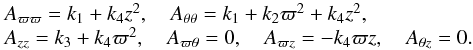 (A.1)Its determinant is
  where k1,k3 are time dependent, positive functions, and k2,k4 non negative constants11.
Similarly, the mean velocity v is obtained from Eqs. (1) and (2). Its components are 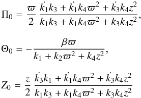 (A.2)with β constant. The dots mean time derivatives. Therefore, a steady state system is only capable of differential rotation.
In the case k ≡ k1 = k3, we get 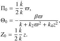 (A.3)
(A.3)
Appendix A.2: Second central moments
The stellar density is obtained with the integration of the phase space density function over the velocity space ΓV,  (A.4)For a Schwarzschild velocity distribution, , we get
  (A.5)Then, the tensor of second central moments, which is defined as
  (A.6)satisfies12
 According to Eq. (A.1), its elements have the following functional dependency,
 ![\appendix \setcounter{section}{1} \begin{equation} \label{moments} \begin{array}{l} \displaystyle \mu_{\varpi \varpi}=\frac{k_3+k_4\varpi^2}{k_1k_3+k_1k_4\varpi^2+k_3k_4z^2} ,\ \mu_{\theta \theta}=\frac{1}{k_1+k_2\varpi^2+k_4z^2},\\[4mm] \displaystyle \mu_{z z}=\frac{k_1+k_4z^2}{k_1k_3+k_1k_4\varpi^2+k_3k_4z^2} ,\ \mu_{\varpi z}=\frac{k_4\varpi z}{k_1k_3+k_1k_4\varpi^2+k_3k_4z^2},\\ ~\\ \displaystyle \mu_{\varpi \theta}=0 ,\quad \mu_{\theta z}=0.\vspace*{-5mm} \end{array} \end{equation}](/articles/aa/full_html/2014/01/aa22436-13/aa22436-13-eq243.png) (A.7)The tilt δ of the velocity ellipsoid, ut·μ-1·u = 1, satisfies
(A.7)The tilt δ of the velocity ellipsoid, ut·μ-1·u = 1, satisfies  (A.8)In the case k ≡ k1 = k3, the above relationship becomes
  (A.9)Then,
  or
or  , so that one of the principal axes of the velocity ellipsoid points towards the GC.
On the other hand, the vertex deviation ε of the velocity ellipsoid satisfies  (A.10)so that, if μϖθ = 0, as in the current axisymmetric case, the vertex deviation is null.
Appendix A.3: Moment gradients
The ϖ and z gradients of the central moments are 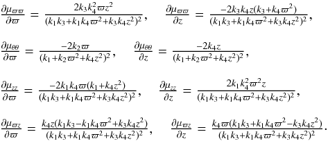 (A.11)Notice that, for z = 0, the values
  , and
, and  are expected to be non-null, in general.
In the GP, the kinematic parameters can be evaluated from the following relationships, 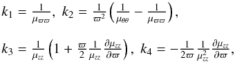 (A.12)which, on the other side, provide the conditions μϖϖ > μθθ,
  , and
, and  .
.
Appendix B: The meaning of U2(0) in the quasi-stationary potential
For a quasi-stationary potential, either in the form of Eq. (31) or in its separable form of Eq. (33), the motion of a star near the GP can be studied by using the reference frame of a circular motion point in the plane. The second equation of motion (e.g., Book I, p. 152) provides the axial component of the angular momentum integral  , while the first equation of motion allows for the description of the radial motion in terms of the effective potential energy
 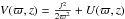 , as
, as  . The circular orbit in the GP satisfies
  and corresponds to a local minimum of V(ϖ,0) at a radius ϖc, satisfying
 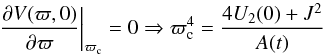 (B.1)under the condition
 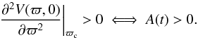 (B.2)Therefore, 4U2(0) + J2 > 0. This is the condition for a stable circular orbit and all the stable non-circular orbits around it. The third equation of motion is consistent with the condition of minimum in z = 0. The circular orbit is a degenerate case of the bounded orbits in its neighbourhood and, from the epicycle approximation, it is possible to prove that they have the same stability as the circular orbit.
In the GP, a repulsive force is associated with a value U2(0) > 0, which allows for stable orbits for all the stars, even for stars with no angular velocity (J = 0), with an oscillating movement along the radial and the vertical directions. This excludes the existence of circular orbits within a radius lower than ![\hbox{$\varpi_{\rm min}=[4U_2(0)/A(t)]^{\frac14}$}](/articles/aa/full_html/2014/01/aa22436-13/aa22436-13-eq271.png) . Otherwise, an attractive force is associated with U2(0) < 0, which allows for bounded orbits only for stars trespassing a threshold angular velocity, with a minimum angular momentum integral
. Otherwise, an attractive force is associated with U2(0) < 0, which allows for bounded orbits only for stars trespassing a threshold angular velocity, with a minimum angular momentum integral  . The other orbits become unstable.
The circular velocity in the plane is given by ![\hbox{$ \displaystyle \Theta_{\rm c}(\varpi)=[A(t)\varpi^2-4U_2(0)\varpi^{-2}]^{\frac12}$}](/articles/aa/full_html/2014/01/aa22436-13/aa22436-13-eq274.png) . For low values of ϖ, if U2(0) < 0, Θc(ϖ) decreases similarly to ϖ-1, while if U2(0) > 0, Θc(ϖ) is null for ϖ < ϖmin and increases for ϖ ≥ ϖmin.
. For low values of ϖ, if U2(0) < 0, Θc(ϖ) decreases similarly to ϖ-1, while if U2(0) > 0, Θc(ϖ) is null for ϖ < ϖmin and increases for ϖ ≥ ϖmin.
Appendix C: Second moments of a n-population mixture
In Cubarsi (1992), Cubarsi & Alcobé (2004), and Pasetto et al. (2012a, 2012b), the velocity moments and cumulants of a two-component mixture were evaluated in terms of the partial statistics and the mean velocity differences between populations. In this appendix, this relationships are generalised to a n-population mixture, by obtaining the total mixture of the second moments in terms of the one-to-one mean velocity differences.
For the ith population, for fixed time and position, let fi represent the velocity distribution function. According to Eq. (A.4), its stellar density is given by  . Each normalised velocity distribution function ψi = fi/Ni defines the respective mean velocity as
  . If the total mixture is written without a subindex and the population fractions are defined as ni = Ni/N, we may obtain the following basic relationships for the normalised density functions, the population fractions, and the mean velocities:
 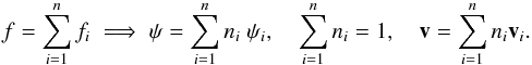 (C.1)The tensor of the second central moments μ, defined in Eq. (A.6), can be expressed working from the population components in terms of the peculiar velocity referred to each population, ui = V − vi, as follows:
 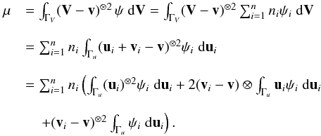 (C.2)Since
  and
and  , by substitution of the mean velocity given in Eq. (C.1), we get
 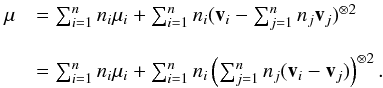 (C.3)We prove the following equality
 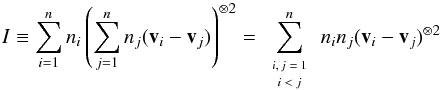 (C.4)by writing I as the addition of the series I1 + I2, so that
 ![\appendix \setcounter{section}{3} \begin{equation} \begin{array}{ll} I&\equiv \sum_{i} n_i \left( \sum_{j\neq i} n_j (\vec v_i-\vec v_j) \right) \otimes \left( \sum_{k\neq i } n_k (\vec v_i-\vec v_k) \right),\\~\\[1.2mm] I_1 &\equiv \sum_{i} n_i \sum_{j\neq i} \sum_{k\neq i,\, k= j } n_j n_k (\vec v_i-\vec v_j) \otimes (\vec v_i-\vec v_k)\\~\\[1.2mm] &=\sum_{i} n_i \sum_{j\neq i} n^2_j (\vec v_i-\vec v_j) ^{\otimes 2}, \\~\\[1.2mm] I_2 &\equiv \sum_{i} n_i \sum_{j\neq i}\sum_{k\neq i, \, k\neq j} n_j n_k (\vec v_i-\vec v_j) \otimes (\vec v_i-\vec v_k). \end{array} \end{equation}](/articles/aa/full_html/2014/01/aa22436-13/aa22436-13-eq296.png) (C.5)The series I1 may be written as13
(C.5)The series I1 may be written as13![\appendix \setcounter{section}{3} \begin{equation} \label{i1} \begin{array}{ll} I_1 &\equiv \sum_{i} \sum_{j> i} (n_i n^2_j +n_j n^2_i) (\vec v_i-\vec v_j)^{\otimes 2}\\~\\[1.2mm] &= \sum_{i} \sum_{j> i} n_i n_j ( n_j +n_i) (\vec v_i-\vec v_j)^{\otimes 2}\\~\\[1.2mm] &= \sum_{i} \sum_{j> i} n_i n_j ( 1- \sum_{k\neq i, \, k\neq j } n_k) (\vec v_i-\vec v_j)^{\otimes 2}\\~\\[1.2mm] &= \sum_{i} \sum_{j> i} n_i n_j (\vec v_i-\vec v_j)^{\otimes 2}- \sum_{i} \sum_{j> i} \sum_{k\neq i, \, k\neq j } n_i n_j n_k (\vec v_i-\vec v_j)^{\otimes 2}. \end{array} \end{equation}](/articles/aa/full_html/2014/01/aa22436-13/aa22436-13-eq298.png) (C.6)Similarly, the series I2 may be written as
(C.6)Similarly, the series I2 may be written as ![\appendix \setcounter{section}{3} \begin{equation} \label{i2} \begin{array}{ll} I_2 &\equiv \sum_{i}\sum_{j\neq i}\sum_{k\neq j,\, k\neq i} n_i n_j n_k (\vec v_i-\vec v_j) \otimes (\vec v_i-\vec v_k)\\~\\ &=\sum_{i}\sum_{j>i}\sum_{k\neq j, \, k\neq i} n_i n_j n_k [(\vec v_i-\vec v_j) \otimes (\vec v_i-\vec v_k) \\~\\ &\quad+ (\vec v_j-\vec v_i) \otimes (\vec v_j-\vec v_k)]\\~\\ &=\sum_{i}\sum_{j>i}\sum_{k\neq j,\, k\neq i} n_i n_j n_k (\vec v_i \otimes \vec v_i - 2 \vec v_i \otimes \vec v_j + \vec v_j \otimes \vec v_j)\\~\\ &=\sum_{i}\sum_{j>i}\sum_{k\neq j, \, k\neq i} n_i n_j n_k (\vec v_i-\vec v_j)^{\otimes 2}. \end{array} \end{equation}](/articles/aa/full_html/2014/01/aa22436-13/aa22436-13-eq300.png) (C.7)
(C.7)
Finally, by addition of Eqs. (C.6) and (C.7) we are led to Eq. (C.4). Then, Eq. (C.3) becomes 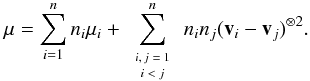 (C.8)Notice, however, that the set of
  differences { (vi − vj) } i,j for i < j are linearly dependent. A reduced set of n − 1 independent quantities is, e.g., { (vk − v1) } k for k > 1, since any difference vi − vj can be obtained as (vi − v1) − (vj − v1).
A mixture of such isothermal distributions in the Galactic plane is also isothermal in the z direction, but is not in the ϖ direction, provided they have different radial mean velocities. Similarly, a mixture of two isotropic distributions in the ϖ and z directions, with different radial mean velocities, is non-isotropic.
As explained in Paper II, Appendix A, this is indeed a consequence of assuming z = 0 as a plane of symmetry for the elements the tensor of covariances and for the mean velocity. If axial symmetry had been the only assumption, the vertex deviation would be null in z = 0, but non-null on either side of the plane.
The above reasoning can also be made as follows. If Eq. (7) is divided by k4, the expression becomes separated into two terms. One of them, Eq. (12), is independent of the population parameters. Then, the other term, Eq. (14), must vanish in order to allow the potential not to depend on the population parameters.

For a generalised Schwarzschild distribution, we get a similar relationship, although multiplied by a factor depending on σ (Cubarsi 2007, Eq. (74)).
References
- Alcobé, S., & Cubarsi, R. 2005, A&A, 442, 929 [NASA ADS] [CrossRef] [EDP Sciences] [Google Scholar]
- Binney, J. 2010, MNRAS, 401, 2318 [NASA ADS] [CrossRef] [Google Scholar]
- Binney, J. 2012, MNRAS, 426, 1328 [NASA ADS] [CrossRef] [Google Scholar]
- Binney, J., & McMillan, P. 2011, MNRAS, 413, 1889 [NASA ADS] [CrossRef] [Google Scholar]
- Bovy, J., Hogg, D. W., & Roweis, S. T. 2009, ApJ, 700, 1794 [NASA ADS] [CrossRef] [Google Scholar]
- Bramich, D. M., Vidrih, S., Wyrzykowski, L., et al. 2008, MNRAS, 386, 887 [NASA ADS] [CrossRef] [Google Scholar]
- Carollo, D., Beers, T. C., Chiba, M., et al. 2010, ApJ, 712, 692 [NASA ADS] [CrossRef] [Google Scholar]
- Casetti-Dinescu, D. I., Girard, T. M., Korchagin, V. I., & van Altena, W. F. 2011, ApJ, 728, 7 [NASA ADS] [CrossRef] [Google Scholar]
- Chandrasekhar, S. 1939, ApJ, 90, 1 [NASA ADS] [CrossRef] [Google Scholar]
- Chandrasekhar, S. 1940, ApJ, 92, 441 [NASA ADS] [CrossRef] [Google Scholar]
- Chandrasekhar, S. 1960, Principles of Stellar Dynamics (New York: Dover Publ. Inc.) [Google Scholar]
- Charlier, C. W. L. 1926, The Motion and the Distribution of the Stars: Memoirs of the University of California, vol. 7 (Berkeley: University of California) [Google Scholar]
- Chiba, M., & Beers, T. C. 2000, AJ, 119, 2843 [NASA ADS] [CrossRef] [Google Scholar]
- Cubarsi, R. 1990, AJ, 99, 1558 [NASA ADS] [CrossRef] [Google Scholar]
- Cubarsi, R. 1992, AJ, 103, 1608 [NASA ADS] [CrossRef] [Google Scholar]
- Cubarsi, R. 2007, MNRAS, 207, 380 [Google Scholar]
- Cubarsi, R. 2010a, A&A, 510, A103 [NASA ADS] [CrossRef] [EDP Sciences] [Google Scholar]
- Cubarsi, R. 2010b, A&A, 522, A30 [NASA ADS] [CrossRef] [EDP Sciences] [Google Scholar]
- Cubarsi, R. 2013, MNRAS, 436, 2874 [NASA ADS] [CrossRef] [Google Scholar]
- Cubarsi, R., & Alcobé, S. 2004, A&A, 427, 131 [NASA ADS] [CrossRef] [EDP Sciences] [Google Scholar]
- Cubarsi, R., & Alcobé, S. 2006, A&A, 457, 537 [NASA ADS] [CrossRef] [EDP Sciences] [Google Scholar]
- Cubarsi, R., Sanz, J., & Juan, J. M. 1990, Ap&SS, 170, 197 [NASA ADS] [CrossRef] [Google Scholar]
- Cubarsi, R., Alcobé, S., Vidojević, S., & Ninković, S. 2010, A&A, 510, A102 [NASA ADS] [CrossRef] [EDP Sciences] [Google Scholar]
- Erickson, R. R. 1975, ApJ, 195, 343 [NASA ADS] [CrossRef] [Google Scholar]
- ESA 1997, The Hipparcos Catalogue, ESA SP-1200 [Google Scholar]
- Famaey, B., Pont, F., Luri, X., et al. 2007, A&A, 461, 957 [NASA ADS] [CrossRef] [EDP Sciences] [Google Scholar]
- Freeman, K., & Bland-Hawthorn, J. 2002, ARA&A, 40, 487 [NASA ADS] [CrossRef] [Google Scholar]
- Fricke, W. 1952, Astron. Nachr., 280, 193 [NASA ADS] [CrossRef] [Google Scholar]
- Fuchs, B., Dettbarn, C., & Rix, H. W. 2009, AJ, 137, 4149 [NASA ADS] [CrossRef] [Google Scholar]
- Girard, T. M., Korchagin, V. I., Casetti-Dinescu, D. I., et al. 2006, AJ, 132, 1768 [NASA ADS] [CrossRef] [Google Scholar]
- Holmberg, J., Nordström, B., & Andersen, J. 2007, A&A, 475, 519 [NASA ADS] [CrossRef] [EDP Sciences] [MathSciNet] [Google Scholar]
- Juan-Zornoza, J. M. 1995, Ph.D. Thesis, Universitat de Barcelona, Spain [Google Scholar]
- Kapteyn, J. C. 1922, ApJ, 55, 302 [NASA ADS] [CrossRef] [Google Scholar]
- Levine, E. S., Heiles, C., & Blitz, L. 2008, ApJ, 679, 1288 [NASA ADS] [CrossRef] [Google Scholar]
- Lynden-Bell, D. 1967, MNRAS, 136, 101 [NASA ADS] [CrossRef] [Google Scholar]
- Moni Bidin, C., Carraro, G., & Méndez, R. A. 2012, ApJ, 747, 101 [NASA ADS] [CrossRef] [Google Scholar]
- Nordström, B., Mayor, M., Andersen, J., et al. 2004, A&A, 418, 989 [NASA ADS] [CrossRef] [EDP Sciences] [Google Scholar]
- Ogorodnikov, K. F. 1965, Dynamics of Stellar Systems (Oxford: Pergamon Press) [Google Scholar]
- Pasetto, S., Grebel, E. K., Zwitter, T., et al. 2012a, A&A, 547, A70 [NASA ADS] [CrossRef] [EDP Sciences] [Google Scholar]
- Pasetto, S., Grebel, E. K., Zwitter, T., et al. 2012b, A&A, 547, A71 [NASA ADS] [CrossRef] [EDP Sciences] [Google Scholar]
- Reid, M. J., Menten, K. M., Zheng, X. W., et al. 2009, ApJ, 700, 137 [NASA ADS] [CrossRef] [Google Scholar]
- Sala, F. 1990, A&A, 235, 85 [NASA ADS] [Google Scholar]
- Sanz-Subirana, J. 1987, Ph.D. Thesis, Universitat de Barcelona, Spain [Google Scholar]
- Siebert, A., Bienaym, O., Binney, J., et al. 2008, MNRAS, 391, 793 [NASA ADS] [CrossRef] [Google Scholar]
- Siebert, A., Williams, M. E. K., Siviero, A., et al. 2011, AJ, 141, 187 [NASA ADS] [CrossRef] [Google Scholar]
- Smith, M. C., Evans, N. W., & An, J. H. 2009a, ApJ, 698, 1110 [NASA ADS] [CrossRef] [Google Scholar]
- Smith, M. C., Evans, N. W., Belokurov, V., et al. 2009b, MNRAS, 399, 1223 [NASA ADS] [CrossRef] [Google Scholar]
- Soubiran, C., & Girard, P. 2005, A&A, 438, 139 [NASA ADS] [CrossRef] [EDP Sciences] [Google Scholar]
- Steinmetz, M. 2012, Astron. Nachr., 333, 523 [NASA ADS] [CrossRef] [Google Scholar]
- Steinmetz, M., Zwitter, T., Siebert, A., et al. 2006, AJ, 132, 1645 [NASA ADS] [CrossRef] [Google Scholar]
- Strömberg, G. 1925, ApJ, 61, 363 [NASA ADS] [CrossRef] [Google Scholar]
- Ting, Y. S., Rix, H. W., Bovy, J., & van de Ven, G. 2013, MNRAS, 434, 652 [NASA ADS] [CrossRef] [Google Scholar]
- Vorobyov, E. I., & Theis, Ch. 2008, MNRAS, 383, 817 [NASA ADS] [CrossRef] [Google Scholar]
- Xue, X. X., Rix, H. W., Zhao, G., et al. 2008, ApJ, 684, 1143 [NASA ADS] [CrossRef] [Google Scholar]
- Zwitter, T., Siebert, A., Munari, U., et al. 2008, AJ, 136, 421 [NASA ADS] [CrossRef] [Google Scholar]
All Tables
Some kinematic observables of the Galaxy are analytically related to the potential cases arising from the conditions of consistency for mixtures.
All Figures
|
Fig. 1 Stellar density of a single population for the harmonic potential (left), for the non-separable quasi-stationary potential (centre), and for the potential separable in addition in cylindrical coordinates (right). |
| In the text | |
|
Fig. 2 Velocity distribution isocontours projected onto the GP for stars with eccentricity up to 0.15 (left) and up to 0.30 (right), both for GCS stars (Cubarsi 2010). |
| In the text | |
|
Fig. 3 Fraction F of kinetic energy (square root) not involved in rotation as a function of the Galactocentric rotation velocities U,V,W for thin disc (green), thick disc (blue), and halo stars (red). |
| In the text | |
Current usage metrics show cumulative count of Article Views (full-text article views including HTML views, PDF and ePub downloads, according to the available data) and Abstracts Views on Vision4Press platform.
Data correspond to usage on the plateform after 2015. The current usage metrics is available 48-96 hours after online publication and is updated daily on week days.
Initial download of the metrics may take a while.