| Issue |
A&A
Volume 561, January 2014
|
|
|---|---|---|
| Article Number | A91 | |
| Number of page(s) | 17 | |
| Section | Interstellar and circumstellar matter | |
| DOI | https://doi.org/10.1051/0004-6361/201322032 | |
| Published online | 09 January 2014 | |
Online material
Appendix A: Convergence and treatment of oscillations
For most of the choices of parameters, the inversion takes about three to four iteration steps for convergence. We have checked that allowing for more steps does not modify significantly the distribution. The results here were obtained after ten iterations. A number of values for the four main parameters, ξ0,ξ1,σ0,σ1 were tested. We show here the results for one favored set of parameters. It corresponds to ξ0 = 30 pc, σ0 = 0.6, ξ1 = 15 pc, and σ1 = 0.8. Our criteria for this choice of parameters are guided by a balance between the quality of the adjustments to the data and a conservative choice of the smoothing lengths. We are also helped by the distribution pattern itself and, in particular, the appearance of elongated radial structures where there are not enough target stars with regard to the used kernel. However, we cannot avoid such radial structures at large distances where targets are missing if we want to keep a kernel appropriate to the nearby regions and uncover the nearby structures. This is illustrated in the Appendix.
Apart from the introduction of new kernels, the updated code now includes a new stage of convergence control. Indeed, in some areas (the problem arose around l = 80° and b = 0°, a direction that corresponds to strong changes in the cloud properties with increasing longitude) the correlation length is large compared to the distances, thus the model has difficulties by fitting strong extinctions which are mixed with weak extinctions at distances much shorter than the correlation length. Under these conditions, the model oscillates from one iteration to the other
between the presence of a strong structure of extinction and the absence of extinction: two solutions are then possible for the model. To avoid these oscillations, at the end of the third iteration, one detects the extinction data, which are farther than three sigma from the model. In fact, the model practically converged in the majority of the areas of the Galaxy, except in the significant areas where the gradients in extinction are particularly important. The data that are farther from the model show the areas where the model cannot reach the data. In this case, one increases the variance of the data by a factor of 2; this allows putting less weight on the data that deviate too much from the model. One starts again this filtering with each new iteration. From a practical point of view, about 300 sightlines are thus filtered in third iteration, from the total of 23 000. This number decreases from one iteration to the next and vanishes at the end of the sixth iteration. After convergence, the estimated model privileges smoothed solutions with low extinction values.
Appendix B: Distribution at large distances: constraint limitations
While the inversion was performed in a 4000 × 4000 × 600 pc3, the scarcity of distant stars results in very low or in null constraints beyond ≃800 pc. In this case the prior distribution is kept unchanged. We show in Fig. B.1 the computed inverted distribution in the Galactic plane up to + or –2 kpc, in order to illustrate the limits of the area that is actually constrained.
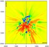 |
Fig. B.1
Galactic plane cut in the 4000 pc 3D distribution of inverted opacity. This map clearly shows the limits between the prior distribution (homogeneous color) and areas where the model has been constrained by the dataset. The elongated radial structures correspond to directions where cavities over dense areas are detected but the number of target stars is too small to constrain their location, hence the spread over a large distance. |
| Open with DEXTER | |
Appendix C: Target distribution
The distribution of the target stars gives the constraints for the inversion. We show in Fig. C.1 those target stars that are located within 10 pc from the plane and have mainly contributed to the computed distribution in this plane, superimposed on the inner part of the computed map. It allows to infer the spatial resolution that can be achieved in a given location. Figure C.2 shows those target stars that are located within 150 pc from the plane and allows to figure out the achievable spatial resolution at larger distance.
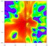 |
Fig. C.1
The Galactic plane cut in the 3D distribution of inverted opacity with stars within 10 pc from the plane superimposed (plus signs). The distribution shows the regions that are well constrained by the data, and how, given the present limited dataset, nearby cavities are better represented than cloud complexes. The distribution also allows the limiting size for the structures to be figured out from the distance between neighboring targets, on the order of 10 pc in the Sun vicinity. |
| Open with DEXTER | |
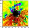 |
Fig. C.2
Same as Fig. C.1, but extending up to 800 pc and displaying stars within 150 pc from the plane. The limiting size for the inverted structures varies from 40 to 200 pc at 800 pc depending on the regions. |
| Open with DEXTER | |
© ESO, 2014
Current usage metrics show cumulative count of Article Views (full-text article views including HTML views, PDF and ePub downloads, according to the available data) and Abstracts Views on Vision4Press platform.
Data correspond to usage on the plateform after 2015. The current usage metrics is available 48-96 hours after online publication and is updated daily on week days.
Initial download of the metrics may take a while.