| Issue |
A&A
Volume 559, November 2013
|
|
|---|---|---|
| Article Number | A78 | |
| Number of page(s) | 18 | |
| Section | Cosmology (including clusters of galaxies) | |
| DOI | https://doi.org/10.1051/0004-6361/201322295 | |
| Published online | 18 November 2013 | |
Online material
Appendix A: Mexican Hat versus FFT spectrum
Since the data cube is non periodic, computing the power spectrum via FFTs is in principle inconsistent. As a consequence, the unresolved large scale power can leak into the available frequency range, distorting the spectrum. We use thus a modified Δ-variance method, known as “Mexican Hat” filtering (MH; cf. Arévalo et al. 2012). For each spatial scale σ, the method consists of three steps:
- 1.
the real-space cube C is convolved with two Gaussian filters having slightly different smoothing lengths:
 and
and  , where ϵ ≪ 1;
 - 2.
the difference of the two cubes is computed, resulting in a cube dominated by the fluctuations at scales ≈σ (the difference of two Gaussian filters is simply the Mexican Hat filter, F(x) ∝ ϵ [1 − x2/σ2] exp [ − x2/2σ2], characterized by a positive core and negative wings);
- 3.
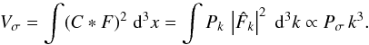
the variance Vσ of the previous cube is calculated and recast into the estimate of the power, knowing that
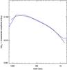 |
Fig. A.1
Comparison of the characteristic amplitude spectra (for the run with M ~ 0.5 and f = 10-2), computed with two different methods: Mexican Hat filtering (black) and fast Fourier transforms (blue). The retrieved spectrum is consistent in both cases, without major differences. |
| Open with DEXTER | |
In Fig. A.1, we show the comparison between the MH and FFT spectrum, for the run with M ~ 0.5 and f ~ 10-2. In our study, there is no dramatic difference between the two methods. The slope in the inertial range is almost identical. At very small scales, the FFT spectrum produces a characteristic hook, in part due to the numerical noise near the maximum resolution, but also due to the contamination of jumps at the non-periodic boundaries. The MH spectrum shows instead a gentle decline. In the opposite regime, the MH filter tends to smooth the scales greater than the injection scale, while the FFT spectrum shows a steeper decrease. The FFT peak is slightly higher, typically by 2−3 percent, likely affected by the non-periodic box. Progressively trimming the box increases the relative normalization of the FFT spectrum, even by 20 percent, while distorting the low-frequency slope; the MH spectrum is instead unaltered.
Appendix B: β-profile in Fourier space
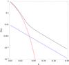 |
Fig. B.1
Analytic 1D power spectra: β-profile (red), Kolmogorov noise (blue), β-profile perturbed by the noise (black; |
| Open with DEXTER | |

We present here the analytic conversion of the β-profile to Fourier space, and its interplay with a power-law noise. Using the notation 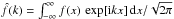 , the Fourier transform of the β-profile (Eq. (1)) results to be
 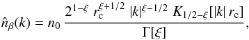 (B.1)where ξ ≡ 3β/2, K1/2 − ξ is a modified Bessel function of the second kind, and Γ is the Gamma function. The (1D) power spectrum is as usual retrieved as
  . Assuming β = 2/3 ≃ 0.66 (a typical value for galaxy clusters), the power spectrum of the β-profile reduces to
 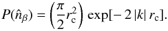 (B.2)The previous equation strikes for its simplicity, and can be readily used in semi-analytic studies. Changing β in the range 0.5−1 does not significantly alter P(k), hence Eq. (B.2) is an excellent approximation for the majority of clusters (Fig. B.1, red line). A remarkable feature is that the transition from real to Fourier space does not dramatically deform the profile, in tight analogy with Gaussian functions (∝exp [ − k2]). The spectrum is dominated by the power on large scales, with the core radius playing a crucial role; a progressively rising rc leads to an increase in both the normalization and steepness of the spectrum.
For our study, it is useful to analyze the superposition of the β-profile and a power-law Kolmogorov noise (with 1D power ∝k− 5/3), np = nβ (1 + δ). Using the convolution theorem, the power spectrum of the perturbed density profile is given by 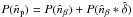 . The cross terms cancel out since the
δ field is random and the phases are uncorrelated. In Fig. B.1, we show three power spectra: β-profile (red), noise with ~10 percent relative amplitude (blue), and the superposition of both (black). Beyond the core radius (k ≳ 0.05), the noise clearly starts to dominate. It is thus not essential to remove the underlying profile or large-scale coherent structures, in order to unveil density perturbations, especially with substantial turbulence.
© ESO, 2013
Current usage metrics show cumulative count of Article Views (full-text article views including HTML views, PDF and ePub downloads, according to the available data) and Abstracts Views on Vision4Press platform.
Data correspond to usage on the plateform after 2015. The current usage metrics is available 48-96 hours after online publication and is updated daily on week days.
Initial download of the metrics may take a while.