| Issue |
A&A
Volume 559, November 2013
|
|
|---|---|---|
| Article Number | A46 | |
| Number of page(s) | 26 | |
| Section | Interstellar and circumstellar matter | |
| DOI | https://doi.org/10.1051/0004-6361/201321171 | |
| Published online | 06 November 2013 | |
Online material
Appendix A: Improvements and changes of the model compared to Bruderer et al. (2012)
Appendix A.1: Continuum radiative transfer
The 3D Monte-Carlo radiative transfer method implemented in the model consists of two stages (see Bruderer et al. 2012, Appendices A.1 and A.2). In the first stage, the dust temperature is obtained using a method combining the algorithm by Bjorkman & Wood (2001) and Lucy (1999). In order to improve the accuracy of the dust temperature in very optically thick midplanes and to speed up the calculation, we have replaced the modified random walk (MRW) approach (Min et al. 2009; Robitaille 2010) by the solution of the diffusion equation. Following a suggestion by Pinte et al. (2009), photon packages are mirrored back from very optically thick regions in the midplane where opacities at the peak wavelength of the star are τ > 1000. At this depth in the disk, the radiation field is close to isotropic and the mean intensity is similar to a black body of the local radiation field. Thus, the diffusion approximation may be employed. After all photon packages have been propagated, the dust temperature in the midplane is obtained from the solution of the diffusion equation 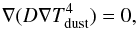 (A.1)where D is the diffusion constant D = 1/(3ρκR(Tdust)), with the Rosseland mean mass extinction coefficient κR(Tdust). The diffusion equation is also used for cells with low photon statistics (see Min et al. 2009).
To verify the changes made in the code, we have re-run the benchmark tests suggested in Pinte et al. (2009) (see Fig. A.3 in Bruderer et al. 2012). As an example, Fig. A.1 shows a comparison of the midplane dust temperature obtained with our updated code and MCFost (Pinte et al. 2006). The model with isotropic scattering and a midplane opacity of τ = 105 is shown. We find very good agreement with deviations comparable to those between other codes tested in the benchmark study. The main improvement to Bruderer et al. (2012) is the reduced calculation time combined with a better accuracy in regions of high opacity or low photon statistics, like regions shielded by a very opaque inner rim.
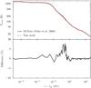 |
Fig. A.1
Disk midplane dust temperature for the disk benchmark problem proposed in Pinte et al. (2009) (τ = 105). The result obtained from our code is given in the red dashed line, the results by MCFost (Pinte et al. 2006) in black. |
| Open with DEXTER | |
The second stage of the Monte-Carlo method calculates mean intensities (Bruderer et al. 2012, Appendix A.2). This part has only been used for FUV wavelengths before. We have updated the code to calculate mean intensities of the entire spectrum from UV to radio wavelengths. We typically use about 60 wavelength bins. The updated code also accounts for photons emitted by the dust. The fraction of photon packages emitted by the protostar, the dust and the interstellar radiation field or cosmic microwave background is chosen according to their relative contribution to the luminosity at one wavelength (e.g. Pinte et al. 2006; Harries 2011).
 |
Fig. A.2
Comparison of the model fluxes between the current model and the representative model of HD 100546 in Bruderer et al. (2012). |
| Open with DEXTER | |
The accuracy of the mean intensity calculated in the second stage can be verified by checking the consistency with the dust temperature obtained in the first stage. We compare the energy balance 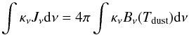 (A.2)using the dust temperature Tdust from the first stage and the mean intensity Jν from the second stage and find agreement to within a few percent. The advantage of splitting the calculation in two stages is that the photons propagating in the first stage mainly sample the peak wavelength of the local radiation field to obtain an accurate dust temperature, while the photons in the second stage are distributed equally between the wavelengths to obtain a well sampled radiation field at all wavelengths. This is important for photodissociation, chemistry, and excitation.
Appendix A.2: Molecular excitation
The main difference between Bruderer et al. (2012) and the present model is the non-LTE calculation of the molecular/atomic excitation. In order to simplify the calculation, we chose to compute the molecular excitation in a 1+1D approach only accounting for the vertical and radial direction to obtain the escape probabilities. The rate coefficient for transitions between level i and j (Eq. (A.17) in Bruderer et al. 2012) is 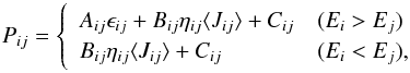 (A.3)with the collisional rate coefficients Cij, the Einstein A and B-coefficients Aij and Bij, respectively and the level energy Ei. The continuum mean intensity ⟨ Jij ⟩ is taken from the Monte-Carlo radiative transfer calculation. The escape probabilities in vertical direction ϵij and radial direction ηij are obtained from (e.g. Avrett & Hummer 1965),
 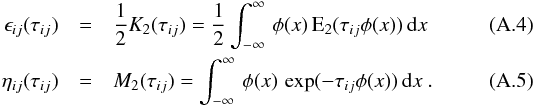 with τij, the line center opacity in vertical or radial direction, respectively. The line profile is taken to be a Doppler line profile function
  and E2(x) is the second exponential integral. The expression for ϵij corresponds to the escape probability of a slab, averaged over angle and line profile and the expression for ηij to the escape probability averaged over the line profile. In order to quickly evaluate the integrals in the above expressions, they are implemented using a Padé-approximation which is accurate to better than 0.1% for the whole opacity range used in the models.
The new approach, which is similar to other 1+1D disk models (e.g. Gorti & Hollenbach 2004; Woods & Willacy 2009; Woitke et al. 2009) has the advantage of including the detailed continuum radiation field from the Monte-Carlo calculation for the radiative pumping of the molecules. Another advantage is that it avoids the iteration over the whole structure in order to solve the thermal-balance problem. This cuts down the calculation time of a single disk model by an order of magnitude down to of order 2 h on a standard desktop computer. The accuracy of a similar approach has been tested by Kamp et al. (2010) who find very small differences between this approach and a full radiative transfer calculation.
Appendix A.3: Raytracing
The raytracing to obtain spectral cubes of the line images has been extended by the contribution of scattered continuum photons to the source function. Also, we have implemented a step-size adjustment along the rays, which avoids that the raytracer takes too small steps in regions where the line does not intersect with the frequency of the current channel due to the velocity profile. This method is similar to the technique implemented in RadLite (Pontoppidan et al. 2009) and speeds up the raytracing considerably.
As an additional test for the raytracing to those reported in Bruderer et al. (2012), we have calculated the emission of a completely optically thin line from a molecule that is only abundant in the inner disk with strong velocity gradients. In this situation, the velocity integrated flux in a beam much larger than the disk can be calculated analytically by summing up the contribution of all cells. We have compared the results of the raytracer with the analytical results and find agreement to within a few percent, independent of the inclination of the disk. We note this is a meaningful benchmark test, as strong velocity gradients in the inner disk require an accurate step-size adjustment along the ray in order not to miss narrow lines (Pontoppidan et al. 2009).
Appendix A.4: Thermal balance
Several small changes have been implemented into the thermal balance calculation:
Line heating/cooling
In order to also account for atomic heating through absorption of UV/optical photons followed by radiative and collisional decay, we have implemented larger model atoms into the non-LTE calculation. Table A.1 provides a list of the implemented atoms and the spectroscopic and collisional rates used. Collisional coefficients with electrons have mostly been taken from the Chianti database (v7.0, Dere et al. 1997). Collisional rates with atomic or molecular hydrogen are missing for Mg ii, Si ii, S ii and Fe ii. For Si ii and Fe ii we use estimated collisional rates by Sternberg & Dalgarno (1995), which however only connect the fine structure levels within the electronic ground state.
The molecular coolants considered in the non-LTE calculation are 12CO, 13CO, C18O, OH, H2O, CN and HCN. For the isotope ratios, we take 12C/13C = 70, 16O/18O = 560 and 18O/17O = 3.2 (Wilson & Rood 1994).
Molecular data has been taken from the LAMDA database (Schöier et al. 2005) except for 12CO, where also ro-vibrational levels are accounted for. The ro-vibrational collisional rates are obtained using the approach by Chandra & Sharma (2001), using the current rates from the LAMDA database for the vibrational ground state.
Considered atomic lines.
Pumping of atomic oxygen by OH photodissociation
We now also account for the population of the 1D levels of atomic oxygen by the photodissociation of OH,  (A.6)Following van Dishoeck & Dalgarno (1984), we assume that ~50% of OH photodissociations lead to O(1D).
H 2 heating/cooling
X-ray heating through H2 ionization (Glassgold & Langer 1973; Meijerink & Spaans 2005) is now also accounted for. For the H2 heating and cooling, we use a model with 15 vibrational levels including the effects of fluorescence and excited formation similar to Sternberg & Dalgarno (1995). Since the previously used rates by Röllig et al. 2006 are fits to this small model, the heating/cooling rates of the two approaches agree very well, except for the case of high temperatures where the 15 level model can cool more efficiently than the two level approach since higher vibrational levels are excited (see Röllig et al. 2006).
Appendix A.5: Chemistry
The chemical network is taken consistently with Bruderer et al. (2012), except that we use the H2 formation rate by Cazaux & Tielens (2004, 2010). An additional reaction for the hydrogen loss of a hydrogenated PAH by a photoreaction,  (A.7)is added. It is set to a rate of 10-8G0 s-1, with G0 the FUV field in units of the interstellar radiation field (Le Page et al. 2001).
To solve for the steady-state abundances, we use an improved version of our globally convergent Newton-Raphson solver (Bruderer et al. 2012). In case this method fails to converge, we use a time-dependent solver. Instead of the DVODE package (Brown et al. 1989), we use the LIMEX package (Ehrig et al. 1999) which was found to be more robust.
Appendix A.6: Testing
As a comparison, we have rerun the representative model of HD 100546 in Bruderer et al. (2012) using the updated model. Line fluxes of both models together with observed line fluxes (Sturm et al. 2010) are given in Fig. A.2. While the atomic fine structure lines of C, C+ and O agree to within 20% between the models, the mid-J and high-J lines of CO show differences of up to a factor of two due to changes in the thermal balance. However, all conclusion made in Bruderer et al. (2012) remain unchanged. As pointed out by Bruderer et al. (2012), the mid-J and high-J CO lines are particularly sensitive on the gas temperature.
Appendix B: Intensity and flux conversions
The conversion between intensity in units of Kelvin (Tν) and flux (Fν) requires the knowledge of the telescope beam. Assuming a Gaussian beam with full width at halve maximum of θFWHM, the solid angle of the beam is  (B.1)thus, the conversion between Tν and Fν is
  (B.2)in units, this is
  (B.3)for frequency/velocity integrated intensities it is
  (B.4)where dν/ν = dv/c has been used. Thus
  (B.5)
(B.5)
Appendix C: Effect of different Rgap and Rcav
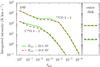 |
Fig. C.1
The representative model with inner disk and dust gap from 10 AU to 45 AU compared to a model with a dust gap from 10 AU to 22.5 AU. Integrated intensities of 12CO 3 − 2 and C18O 3 − 2 inside the gap (r = 16.25 AU) and in the outer disk (r = 100 AU) are shown. |
| Open with DEXTER | |
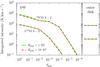 |
Fig. C.2
The representative model with inner disk and dust gap from 10 AU to 45 AU compared to a model with a dust gap from 1 AU to 45 AU. Integrated intensities of 12CO 3 − 2 and C18O 3 − 2 inside the gap (r = 28 AU) and in the outer disk (r = 100 AU) are shown. |
| Open with DEXTER | |
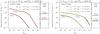 |
Fig. D.1
Integrated intensities of 12CO 3 − 2 at the center of the gap (r = 28 AU) and in the outer disk (r = 100 AU) for different X-ray luminosities (LX), stellar bolometric luminosities (Lbol) and effective temperatures (Teff). The considered range of the X-ray spectrum is given in brackets (either 0.1−10 keV or 1−100 keV). Note that the lines in the left panel lie ontop of each other. |
| Open with DEXTER | |
In order to study the effect of a different cavity size (Rcav in Fig. 1a) and extent of the inner disk (Rgap in Fig. 1a), we have calculated the representative model also with a dust gap extending from 1 AU to 45 AU (Rgap = 1 AU instead of 10 AU) and 10 AU to 22.5 AU (Rcav = 22.5 AU, instead of 45 AU). The resulting integrated intensities in the gap and outer disk are shown Figs. C.1 and C.2 in the same way as Fig. 12. In Fig. C.1 we present the integrated intensity in the center of the smaller cavity, at 16.25 AU (see Sect. 6.1.1).
Models with a smaller cavity radius (smaller Rcav) result in similar integrated intensities at a given radius inside the cavity, with differences <40%. This results from the fact that a point at a certain radius is much more affected by positions at smaller radii than at larger radii, because of the stellar heating and photodissociating radiation coming from inside. We conclude that calculations with smaller cavities are necessary for a detailed modeling, but the trends found from the 45 AU gap also hold for smaller gaps.
Models with a smaller inner disk (smaller Rgap) yield almost same integrated intensity profile inside the cavity, because the inner wall of the inner disk absorbs the stellar heating and photodissociating FUV radiation. This can be seen in Fig. 4d, showing the local FUV radiation. We conclude that the size of the inner disk is not a key parameter, as long as its inner wall can shield the stellar radiation.
Appendix D: Dependence on X-rays
The effect of X-ray radiation on the CO integrated intensity mainly depends on the X-ray luminosity (LX) compared to the FUV luminosity (LFUV). Figure D.1 shows the 12CO 3 − 2 and C18O 3 − 2 integrated intensity for models with dusty inner disk present and Lbol = 10 L⊙, Teff = 10 000 K or Lbol = 1 L⊙, Teff = 6000 K. The latter is the model with the highest LX/LFUV ~ 1 in our grid. However, even this model only shows a change of the 12CO integrated intensity in the gap with the X-ray luminosity, if the amount of gas in the cavity is low (δgas ≲ 10-5). This is because the heating of the upper layers in the gap is dominated by different effects (Sect. 3.1), while deeper in the disk, shielding by the inner disk is sufficient to render X-ray heating less important. The effect of X-rays does not change if the energy range of the thermal spectra is shifted to 0.1−10 keV instead of 1−100 keV. The rare isotopologue C18O shows the same dependence on the X-rays as 12CO. Stellar X-rays are thus not an important parameter for the low-J CO lines.
© ESO, 2013
Current usage metrics show cumulative count of Article Views (full-text article views including HTML views, PDF and ePub downloads, according to the available data) and Abstracts Views on Vision4Press platform.
Data correspond to usage on the plateform after 2015. The current usage metrics is available 48-96 hours after online publication and is updated daily on week days.
Initial download of the metrics may take a while.