| Issue |
A&A
Volume 559, November 2013
|
|
|---|---|---|
| Article Number | A39 | |
| Number of page(s) | 10 | |
| Section | Stellar atmospheres | |
| DOI | https://doi.org/10.1051/0004-6361/201220816 | |
| Published online | 01 November 2013 | |
Online material
Appendix A: Theoretical developments
Appendix A.1: General expression of the PDS
We establish here our general expression of the PDS, that it is Eqs. (7) and (8). We start from the term of Eq. (6), which enters in the RHS of Eq. (1). We apply the operator given by Eq. (2) on Eq. (6), it gives 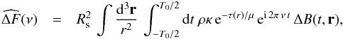 (A.1)where the space integration is performed over half of the (stellar) sphere, d3r = −dμ r2 dr dφ, and dτ = κ ρ.
The extent of the region where the stellar granulation is seen is very small compared to the stellar radius Rs, such that r is almost constant over the optical depth range relevant for calculating the flux. Therefore, in very good approximation we have  in the integrand of Eq. (A.1). Accordingly, Eq. (A.1) can be simplified as
 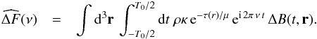 (A.2)Since
  cannot be evaluated in a deterministic way but a statistical one only, we consider the square of Eq. (A.2) and average it over a large number of independent realizations. This gives
 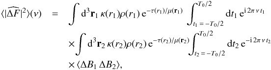 (A.3)where ΔB1 (resp. ΔB2) corresponds to the quantity ΔB evaluated at the time-space position (t1,r1) (resp. (t2,r2)).
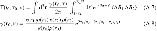
We then define the following new coordinates 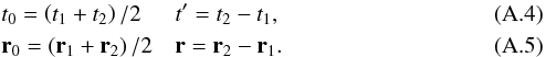 In these coordinates, r and t′ are the spatial correlation and temporal correlation lengths associated with the local properties of the turbulence, while r0 and t0 are mean space and time positions. Using the new coordinates given by Eqs. (A.4) and (A.5) in Eq. (A.6) leads to
 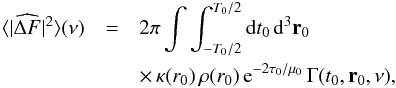 (A.6)where
 and τi = τ(ri),μi = μ(ri) with i = { 0,1,2 }.
At this stage, a tractable expression for Eq. (A.6) calls for more assumptions. We assume that T0 is much longer than the granule lifetime. We neglect length-scales longer than the granulation length-scales. In that case ΔB represents the instantaneous difference between the brightness of the granules situated at the position (τ(r),μ,φ) and the brightness of the material in the steady state (< B > t). Accordingly, Eq. (A.6) reduces to 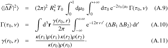 We now assume that κρ varies at a length-scale longer than the characteristic size of the granules. This assumption is discussed in Appendix B. Accordingly, γ ≃ κ(r0)ρ(r0) and Γ reduces to
  (A.12)where
  is the space and time Fourier transform of ⟨ ΔB1 ΔB2 ⟩, defined as
 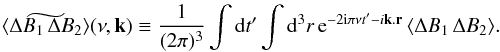 (A.13)Note that, from now on, we substitute the notation τ0 by τ.
We now turn to the time-averaged flux ⟨ F ⟩ t. From Eqs. (3), (4), and (5) one derives  (A.14)where we have defined
  (A.15)Finally, using Eq. (A.9), Eq. (A.12) and Eq. (A.14) we derive the general expressions of Eqs. (7) and (8). The term ℱτ (Eq. (8)) stands for the PDS of the granulation as it would be seen at the optical depth τ. However, the observed PDS associated with the granulation background is given by Eq. (7) and corresponds to the sum of the spectra seen at different layers in the atmosphere, but weighted by the term e− 2τ/μ ( ⟨ B ⟩ t/F0)2.
Appendix A.2: Source function (⟨ ΔB1 ΔB2 ⟩)
To proceed we need to derive an expression for the correlation product ⟨ ΔB1 ΔB2 ⟩. To this end, we recall that B = σT4/π, where σ is the Stefan-Boltzmann constant, and introduce ΔT as the difference between the temperature of the granule and that of the surrounding medium. We thus have  (A.16)where Θ ≡ ΔT/ ⟨ T ⟩ t. The second-order Taylor expansion of the RHS of Eq. (A.16) gives
  (A.17)We have neglected the third and fourth order terms in Θ. Indeed, a 3D hydrodynamical simulation of the solar surface shows that terms higher than second order contribute less than about 15% of Eq. (A.16). Accordingly,
 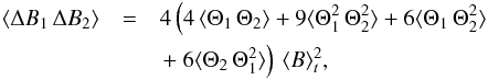 (A.18)where Θ1 ≡ Θ(r1,t1) and Θ2 ≡ Θ(r2,t2).
We now adopt the quasi-normal approximation (QNA). This approximation is rigorously valid for normally distributed quantities. Departure from this approximation is discussed in Appendix B. Normally distributed quantities are necessarily symmetric, such that  and
and  . This approximation also implies (e.g., Lesieur 1997, Chap. VII-2)
 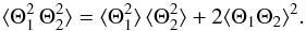 (A.19)The first term in the RHS of Eq. (A.19) does not contribute in the time Fourier domain, except at the null frequency. Accordingly,
  (A.20)Now using the Parseval-Plancherel relation, Eq. (A.20) becomes
  (A.21)with
  (A.22)where ν′′ = ν + ν′ and k′′ = k + k′.
We assume that the scalar Θ is isotropic. Accordingly, the spatial Fourier transform of ⟨ Θ1Θ2 ⟩ (r,ν) is given by (see e.g. Lesieur 1997, Chap. V-10) 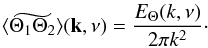 (A.23)The scalar spectrum EΘ(k,ω) is related to the scalar variance as (Lesieur 1997, Chap. V-10)
 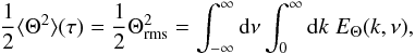 (A.24)where Θrms is by definition the rms of Θ, which is related to ΔTrms (the rms of ΔT) according to
  (A.25)Following Stein (1967), the scalar energy spectrum EΘ(k,ν) can be factorized into a spatial spectrum EΘ(k) and a frequency-dependent factor χk(ν) according to
  (A.26)where the frequency-dependent factor χk(ν) is normalized such that
  (A.27)
Appendix A.3: Final expression of relative flux variations
The final expression for the term ℱτ (Eq. (8)) that appears in the RHS of Eq. (7) is obtained by inserting Eq. (A.21) to (A.23) into Eq. (8), so that  (A.28)where the two terms in the RHS of Eq. (A.28) are considered for (τ,ν,k = 0).
Equation (A.28) can be further simplified by assuming that the temperature fluctuations behave as a passive scalar (see Appendix A.4.1 and the discussion in Appendix B). In that case, it can been shown that the first term in the RHS of Eq. (A.28) vanishes (see Monin & Yaglom 1971, Chap. 14.5). Accordingly, Eq. (A.28) simplifies as  (A.29)with
 The final expression, Eq. (A.29), is recast to a more suitable form. To this end, we define the characteristic wave-number k0 = 2π/Λ where Λ is a characteristic length. We also define the characteristic frequency ν0 = 1/(2π τc) where τc is a characteristic time. Eventually, Eq. (A.29) leads to Eqs. (9), (10) where we have defined the dimensionless source function
  (A.32)as well as the following dimensionless quantities:
 where we have defined the characteristic wavenumber k0 = 2π /Λ, and the characteristic frequency ν0 = 1/(2π τc), where τc ≡ 1/(k0 u0) is a characteristic time and u0 a characteristic velocity (see Eq. (A.40) below). Note that the dimensionless quantities
  and
and  verify the following normalization conditions:
 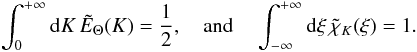 (A.37)
Appendix A.4: Turbulence modeling
Appendix A.4.1: Spatial spectrum
As already mentioned, it is assumed that the temperature fluctuations behave as a passive scalar (see the discussion in Appendix B). Therefore EΘ(k) is given according to (see Lesieur 1997, Chap. VI-10) 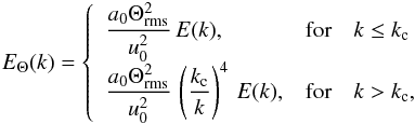 (A.38)where a0 is a normalization factor, E(k) the kinetic energy spectrum, u0 a characteristic velocity (see Eq. (A.40) below), and kc the wavenumber, which separates two characteristic ranges:
-
the inertial-convective range(k < kc). In this domain, advection of the temperature fluctuations by the turbulent velocity field dominates over the diffusion.
-
the inertial-conductive range (k > kc). In this domain, the diffusion of the temperature fluctuations dominates over advection.
We consider for E(k) the Kolmogorov spectrum, and the characteristic velocity u0 is defined such that 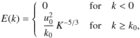 (A.39)where the characteristic velocity u0 is defined such that
 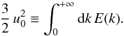 (A.40)From Eq. (A.38) and Eq. (A.39), the spacial spectrum finally becomes
 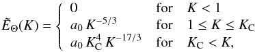 (A.41)where we have defined KC = kc/k0.
Some prescriptions are required for kc and k0. 3D RHD show that from one stellar 3D model to another, the granule size Λ scales approximately as the pressure scale-height (Hp) at the photosphere (Freytag et al. 1997). Accordingly, we assume that 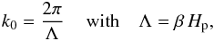 (A.42)where Λ is a characteristic length-scale, Hp the pressure scale height and β is a free parameter. Concerning the characteristic wavenumber kc, in a medium with very low Prandtl number (which is the case in the stellar medium), kc is given by (see Lesieur 1997, Chap. VI)
 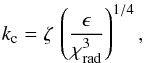 (A.43)where ζ is a free parameters introduced to exercise some control on this prescription, χrad is the radiative diffusivity coefficient, and ϵ is the rate of injection of kinetic energy into the turbulent cascade. The latter is estimated according to
  , where we have introduced the anisotropy factor
 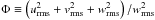 , where urms, vrms, and wrms are the rms of the three components of the velocity (horizontal and vertical ones).
Appendix A.4.2: Frequency spectrum
Since in the inertial-convective range (i.e., k < kc) temperature fluctuations are dominated by advection, we assume that – at this scale range – χk(ν) is the same as the frequency spectrum associated with the velocity field,  . This hypothesis tends to be supported by large eddies simulations (see e.g. Samadi et al. 2003a). Indeed, using a solar hydrodynamic simulation, Samadi et al. (2003a) have found that this property is rather well verified by the entropy fluctuations. Since entropy fluctuations are mostly dominated by temperature fluctuations, this must be the same for the temperature fluctuations. For the inertial-conductive range (k > kc): temperature fluctuations are no longer dominated by advection. However, to our knowledge, no study has been conducted yet about the properties of χk in this range. Therefore, we assume by default that in this range χk varies with ν, as do .
In a strongly turbulent medium, is well described by a Lorentzian function (Sawford 1991; Samadi et al. 2003a; Belkacem et al. 2010), i.e., 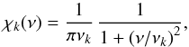 (A.44)where νk is by definition the half-width at half-maximum of χk(ν). In the framework of the Samadi & Goupil (2001) formalism, this latter quantity is evaluated as
  (A.45)with
  (A.46)where λ is a free parameter introduced, following Balmforth (1992), to have some control on the adopted definition for νk. We define the characteristic time τc ≡ 1/(k0 u0), which corresponds to an estimate of the lifetime of the largest eddies. Accordingly, we have ν0 = (2πτc)-1.
The Lorentzian χk (Eq. (A.44)) has a justification for a strongly turbulent medium. However, Georgobiani et al. (2006) have found on the basis of a 3D RHD solar model that χk decreases more rapidly with ν near the photosphere than it does in deeper layers. Accordingly, as an alternative for a Lorenztian function and following Musielak et al. (1994), we also consider for χk an exponential form 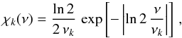 (A.47)where νk is the half-width at half-maximum. We alternatively adopted here the two different prescriptions for χk.
Appendix B: Approximations and assumptions
Our theoretical model is based on three major approximations and assumptions. They are discussed below.
Passive scalar assumption: it was assumed that the temperature fluctuations behave as a passive scalar. We recall that a passive scalar is a quantity that obeys an equation of diffusion (e.g., Lesieur 1997). For the temperature fluctuations, this equation of diffusion is rigorously valid when the diffusion and the Boussinesq approximations are verified and the stratification is negligible compared with the eddy size. However, all these conditions are not fulfilled in the vicinity of the photosphere where the granules are the more visible. Indeed, in this region the medium is optically thin such that the diffusion approximation does no longer hold. Furthermore, this region is characterized by a non-negligible turbulent Mach number that prevents the Boussinesq approximation from being valid. Finally, the granule sizes are typically of the order of the pressure-scale height (see below). Nevertheless, as shown by Espagnet et al. (1993) and Hirzberger et al. (1997), the spectrum, EΘ, associated with the temperature fluctuations at the surface of the Sun scales with k as predicted by Eq. (A.38), which was derived assuming that the temperature fluctuations behave as a passive scalar. This suggests that somehow the temperature fluctuations obey an equation of diffusion.
Quasi-normal approximation (QNA): the approximation of Eq. (A.19) assumes that fluctuating quantities are distributed according to a normal distribution. However, it is well known that the departure from the QNA is important in a strongly turbulent medium (Ogura 1963). Furthermore, the upper-most part of the convection zone is a turbulent convective medium composed of essentially two flows (the granules and the downdraft plumes) that are asymmetric with respect to each other. Therefore, we obviously do not deal with symmetric distribution, as it is the case for a normal distribution. With the help of a solar 3D hydrodynamical simulation, Belkacem et al. (2006) have quantified the departure from the QNA (seee also Kupka & Robinson 2007). However, by comparing 3D hydrodynamical models representative of different main-sequence stars, we have found that this departure does not vary significantly across the main sequence.
Length-scale separation: the derivation of Eq. (7) is based on the assumption that the product κρ varies at a length-scale significantly longer than the granule size. However, in the case of the Sun, for instance, the granules have a size of about 2 Mm (see e.g. Muller 1989; Roudier et al. 1991) while the pressure-scale height, Hp, is of the order of few hundred kilometers at the photosphere. Because near the photosphere the density scale-height Hρ is of the same order as Hp and even lower, our assumption does not hold near the photosphere. Nevertheless, 3D hydrodynamic models show that from a stellar model to another, the granule size scales as the pressure scale-height at the photosphere (Freytag et al. 1997; Samadi et al. 2008). Therefore, as for the QNA, we expect that the departure from our hypothesis introduces a bias that remains almost constant across the Hertzsprung-Russell diagram.
The major approximations and assumptions adopted in our model are expected to be in default near the photosphere. However, avoiding these approximations and assumptions would require additional theoretical improvements, and they constitute – at the present time – the only way for deriving an analytical model of the granulation spectrum. We also recall that our objective is to derive a simple analytical model for the interpretation of the observed scaling relations. Furthermore, provided that the three free parameters involved in the model are appropriately tuned, the theoretical model agrees reasonably well with the Ludwig (2006) 3D hydrodynamical approach (see Sect. 4).
Appendix C: Eddy-time correlation
Two different functions for χk(ν) were tested: a Lorentzian function and an exponential one. For a strongly turbulent medium, one expects a Lorentzian function (Sawford 1991; Samadi et al. 2003a; Belkacem et al. 2010). However, with this function, the theoretical granulation spectrum decreases as ν-2, while the observations decreases much more rapidly with ν. On the other hand, adopting an exponential χk results in a much better agreement at high frequency. This is because an exponential χk decreases more rapidly with frequency than does a Lorenztian χk. Finally, as in the Sun, adopting an exponential χk results in a much better match with the theoretical PDS computed with the ab initio approach for two 3D hdyrodynamical models, one representative for an F-type star and the other one for a red giant star (see Sect. 4).
According to Sawford (1991, see also Appourchaux et al. 2010, the time-Fourier transform of the Lagrangian eddy-time
correlation function is expected to tend to a Lorentzian function when the Reynolds number tends to infinity. In contrast, the less turbulent the medium (i.e., in general the lower Reynolds number), the more rapid the decrease of χk with increasing ν. This behavior is also supported for the Eulerian eddy-time correlation (χk) by hydrodynamical numerical models (see e.g. Samadi 2011). In other words, the ν variation of χk is expected to depend on the degree of turbulence. Accordingly, our result confirms that the granules, which are mainly visible near the photosphere, are less turbulent than the super-adiabatic layers situated a few hundred kilometers below the photosphere. We therefore confirm the previous claim by Nordlund et al. (1997) that the granules have a low level of turbulence. This is also consistent with the results by Georgobiani et al. (2006, see also Nordlund et al. 2009. Indeed, these authors showed that χk decreases more rapidly with ν near the surface of a solar 3D model than it does in deeper layers, where χk is close to a Lorentzian function (Samadi et al. 2003a).
Finally, the fact that the granules have a relatively low level of turbulence is probably not specific to the Sun. Indeed, the 3D RHD models of stars show that the granules have similar properties as in the Sun (e.g., Trampedach et al. 2013). Therefore, it is not surprising that the theoretical PDS computed with the ab initio approach varies with ν in a similar way as in the Sun.
Appendix D: Remaining discrepancies
Although globally satisfactory, the theoretical model does not reproduce the solar granulation spectrum perfectly. Indeed, the observed spectrum shows a kink at ν ~ 1 mHz (see Sect. 3.2). There is no consensus yet about the physical origins of this feature. Depending on the authors, it is either attributed to the occurrence of bright points (e.g., Harvey et al. 1993; Aigrain et al. 2004), the changing properties of the granules (Andersen et al. 1998), a second granulation population (Vázquez Ramió et al. 2005), and finally to faculae (Karoff 2012). A similar discrepancy was obtained by Ludwig et al. (2009) on the basis of the ab initio approach. This indicates that pure hydrodynamical approaches cannot fully account for the observed solar granulation spectrum. Nevertheless, the remaining discrepancies represent only a small fraction of the total brightness fluctuations produced by the granulation phenomenon.
The theoretical model does not perfectly reproduced the PDS obtained with the ab initio approach for the two 3D models considered in this work. For instance, a difference of less than about 15% is obtained for σ with the 3D model for an F-dwarf star and a difference less than about 30% are obtained for τeff with the 3D model for a red giant star. These differences must be attributed to the different approximations and assumptions adopted (see Appendix B above). Nevertheless, they remain of the order of the dispersion obtained between the different methods of analysis investigated by Mathur et al. (2011, see also Paper II). Because the ab initio modeling is based on a very limited set of physical hypothesis, the reasonable agreement between the two approaches shows that despite the numerous hypotheses and assumptions adopted in our theoretical model (see Appendix B), our model provides realistic results.
© ESO, 2013
Current usage metrics show cumulative count of Article Views (full-text article views including HTML views, PDF and ePub downloads, according to the available data) and Abstracts Views on Vision4Press platform.
Data correspond to usage on the plateform after 2015. The current usage metrics is available 48-96 hours after online publication and is updated daily on week days.
Initial download of the metrics may take a while.