| Issue |
A&A
Volume 557, September 2013
|
|
|---|---|---|
| Article Number | A53 | |
| Number of page(s) | 20 | |
| Section | Astrophysical processes | |
| DOI | https://doi.org/10.1051/0004-6361/201321160 | |
| Published online | 28 August 2013 | |
Online material
Appendix A: Harmonic-domain CCA
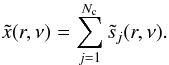
The sky radiation,  ,
from direction r at frequency ν results from the
superposition of signals coming from Nc different physical
processes
,
from direction r at frequency ν results from the
superposition of signals coming from Nc different physical
processes  :
:
 (A.1)The
signal
is observed through a telescope, the beam pattern of which can be modelled at each
frequency as a spatially invariant point spread function
B(r,ν). For each value of ν, the
telescope convolves the physical radiation map with B. The
frequency-dependent convolved signal is input to an
Nd-channel measuring instrument, which integrates the signal
over frequency for each of its channels and adds noise to its outputs. The output of the
measurement channel at a generic frequency ν is
(A.1)The
signal
is observed through a telescope, the beam pattern of which can be modelled at each
frequency as a spatially invariant point spread function
B(r,ν). For each value of ν, the
telescope convolves the physical radiation map with B. The
frequency-dependent convolved signal is input to an
Nd-channel measuring instrument, which integrates the signal
over frequency for each of its channels and adds noise to its outputs. The output of the
measurement channel at a generic frequency ν is 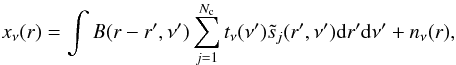 (A.2)where
tν(ν′) is the
frequency response of the channel and
nν(r) is the noise map.
The data model in Eq. (A.2) can be
simplified by virtue of the following assumptions:
(A.2)where
tν(ν′) is the
frequency response of the channel and
nν(r) is the noise map.
The data model in Eq. (A.2) can be
simplified by virtue of the following assumptions:
-
Each source signal is a separable func-tion of direction and frequency, i.e.,
 (A.3)
(A.3) -
B(r,ν) = Bν(r)is constant within the bandpass of the measurement channel.
These two assumptions lead us to a new data model: 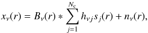 (A.4)where
∗ denotes convolution, and
(A.4)where
∗ denotes convolution, and  (A.5)For
each location, r, we define
(A.5)For
each location, r, we define
-
the Nc-vector s (sources vector), whose elements are sj(r);
-
the Nd-vector x (data vector), whose elements are xν(r);
-
the Nd-vector n (noise vector), whose elements are nν(r);
-
the diagonal Nd-matrix B, whose elements are Bν(r);
-
the Nd × Nc matrix H, containing all hνj elements.
Then, we can rewrite Eq. (A.4) in
vector form:  (A.6)The
matrix H is called the mixing matrix and contains the frequency
scaling of the components for all the data maps involved.
(A.6)The
matrix H is called the mixing matrix and contains the frequency
scaling of the components for all the data maps involved.
Under the assumption that B does not depend on the frequency,
when working in the pixel domain, we can simplify Eq. (A.6) to  (A.7)where
the components in the source vector s are now convolved
with the instrumental beam.
(A.7)where
the components in the source vector s are now convolved
with the instrumental beam.
Equation (A.6) can be translated into
the harmonic domain, where for each transformed mode it becomes  (A.8)where
X, S, and
N are the transforms of
x, s, and
n, respectively, and
(A.8)where
X, S, and
N are the transforms of
x, s, and
n, respectively, and
 is the
transform of matrix B. Relying on this data model, we can
derive the following relation between the cross-spectra of the data
is the
transform of matrix B. Relying on this data model, we can
derive the following relation between the cross-spectra of the data
 ,
sources
,
sources
 and
noise,
and
noise,
 , all
depending on the multipole ℓ:
, all
depending on the multipole ℓ:
 (A.9)where
the dagger superscript denotes the adjoint matrix. To reduce the number of unknowns, the
mixing matrix is parametrized through a parameter vector p
(such that
H = H(p)),
using the fact that its elements are proportional to the spectra of astrophysical
sources (see Sect. 3.2).
(A.9)where
the dagger superscript denotes the adjoint matrix. To reduce the number of unknowns, the
mixing matrix is parametrized through a parameter vector p
(such that
H = H(p)),
using the fact that its elements are proportional to the spectra of astrophysical
sources (see Sect. 3.2).
Since the foreground properties are expected to be spatially variable, we work on relatively small square patches of data. This allows us to use the 2D Fourier transform to approximate the harmonic spectra (see, e.g., Bond & Efstathiou 1987).
The HEALPix (Górski et al. 2005) data on the
sphere are projected on the plane tangential to the centre of the patch and are
re-gridded with a suitable number of bins to correctly sample the original resolution.
Each pixel in the projected image is associated with a specific vector normal to the
tangential plane and assumes the value of the HEALPix pixel nearest to the corresponding
position on the sphere. Clearly, the projection and re-gridding process will create some
distortion in the image at small scales and will modify the noise properties. However,
we verified that this has only a negligible impact on the spectra in Eq. (A.9) for the scales considered in this work
and, therefore, on the spectral parameters. If
x(i,j) contains the data projected on
the planar grid and X(i,j) is its
two-dimensional discrete Fourier transform, the energy of the signal at a certain scale,
which corresponds to the power spectrum, can be obtained as the average of
X(i,j)X†(i,j)
over annular bins  ,
,
 (Bedini & Salerno 2007):
  (A.10)where
 is the number of pairs (i,j) contained in the spectral bin denoted by
.
Every spectral bin
is the number of pairs (i,j) contained in the spectral bin denoted by
.
Every spectral bin  is related to a specific ℓ in the spherical harmonic domain by
 (A.11)where
p is the thickness of the annular bin,
Δℓ = 180/Ldeg(Npix − 1),
and Ldeg, Npix are the size in
degrees and the number of pixels on the side of the square patch, respectively.
(A.11)where
p is the thickness of the annular bin,
Δℓ = 180/Ldeg(Npix − 1),
and Ldeg, Npix are the size in
degrees and the number of pixels on the side of the square patch, respectively.
If we reorder the matrices  and
and  into vectors
  and
and  ,
respectively, we can rewrite Eq. (A.9)
as
,
respectively, we can rewrite Eq. (A.9)
as  (A.12)where
 , and the symbol ⊗ denotes the
Kronecker product. The vector
, and the symbol ⊗ denotes the
Kronecker product. The vector  is now computed using the approximated data cross-spectrum matrix in Eq. (A.10) and
 represents the error on the noise power spectrum.
The parameter vector p and the source cross-spectra are
finally obtained by minimizing the functional 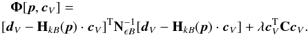 (A.13)The
vectors dV and
cV contain the elements
and ,
respectively, and the diagonal matrices
HkB and
Nϵ the elements
(A.13)The
vectors dV and
cV contain the elements
and ,
respectively, and the diagonal matrices
HkB and
Nϵ the elements
 and the covariance of error
  for all relevant spectral bins. The term
  is a quadratic
stabilizer for the source power cross-spectra: the matrix C is
in our case the identity matrix, and the parameter λ must be tuned to
balance the effects of data fit and regularization in the final solution. The functional
in Eq. (A.13) can be considered as a
negative joint log-posterior for p and
cV, where the first
quadratic form represents the log-likelihood, and the regularization term can be viewed
as a log-prior density for the source power cross-spectra.
is a quadratic
stabilizer for the source power cross-spectra: the matrix C is
in our case the identity matrix, and the parameter λ must be tuned to
balance the effects of data fit and regularization in the final solution. The functional
in Eq. (A.13) can be considered as a
negative joint log-posterior for p and
cV, where the first
quadratic form represents the log-likelihood, and the regularization term can be viewed
as a log-prior density for the source power cross-spectra.
Appendix B: Spectral model for AME
Theoretical spinning-dust models predict a variety of spectra that can be substantially different in shape, depending on a large number of parameters describing the physics of the medium. The number of these physical parameters is too large to be constrained by the data in the available frequency range. For the purpose estimating the spectral behaviour of the AME we adopted a simple formula depending on only a few parameters. The CCA component-separation method used in this work implements the parametric relation proposed by Bonaldi et al. (2007) (Eq. (6)), depending on the peak frequency, νp, and slope at 60 GHz, m60. To verify the adequacy of this parametrization we produced spinning-dust spectra for different input physical parameters with the SpDust code and fitted each of them with the proposed relation by minimizing the χ2 for the set of frequencies used in this work. The input models we considered are weak neutral medium (WNM), cold neutral medium (CNM), weak ionized medium (WIM), and molecular cloud (MC). Both the input SpDust parameters and the best-fit m60, νp parameters for each model are reported in Table B.1. For comparison, we also considered alternative parametric relations and in particular
-
the model implemented in the Commander componentseparation method (Pietrobonet al. 2012; PlanckCollaboration 2013d) which is a Gaussian in the TCMB − ln(ν)plane, parametrized in terms of central frequency and width;
-
the Tegmark et al. (2000) model, which is a modified black-body relation (Eq. (1)) with a temperature of around 0.25K and an emissivity index of about 2.4;
Because this test neither accounts for the presence of the other components and includes any data simulation, it verifies the intrinsic ability of the parametric model to reproduce the actual spectra. Realistic estimation errors for the CCA model are derived through simulations in Appendix C.
Figure B.1 compares the input spectra with the best-fit models for the different parametrizations. In general, the fits are accurate at least up to ν = 50–60 GHz, while at higher frequencies the parametric relations may not be able to reproduce the input spectra in detail. This is a consequence of fitting complex spectra with only a few parameters. The fit tends to fail where the AME signal is weaker.
Over the frequency range considered, CCA and Commander models fit the input spectrum generally better than the Tegmark et al. (2000) model (which decreases too rapidly at high frequencies). When adding lower frequency data, however, CCA and Commander models will be increasingly inaccurate, because they are symmetric with respect to the peak of the emission. The models implemented by CCA and Commander perform quite similarly, despite the different formulation. As a result, these methods are able to give consistent answers, which ensures consistency between different analyses within Planck (e.g. Planck Collaboration 2013d).
The CCA model used in this work provides a reasonable fit to theoretical spinning-dust models for a variety of physical conditions. The best-fit parameters that we obtain, reported in Table B.1, vary significantly from one input model to another and have a straightforward interpretation in terms of the spectrum.
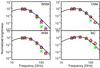 |
Fig.B.1
Theoretical spinning dust models produced with SpDust (solid lines) and fitted with CCA (triangles), Commander (diamonds), and Tegmark et al. (2000) (asterisks) models. Input SpDust parameters and best-fit parameters for the CCA model are provided in Table B.1. |
| Open with DEXTER | |
Appendix C: Description of the simulations
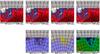 |
Fig.C.1
Free-free templates at 23 GHz used for the analysis. The reference template FFREF is in the upper left corner; the other columns (left to right) are FF1, FF2 and FF3, respectively. The differences in the lower panels (FFi − FFREF)/FFREF are on average of the order of 10%, but reach 50% in regions of strong dust emission. |
| Open with DEXTER | |
We simulated Planck and WMAP 7-yr data by assuming monochromatic bandpasses positioned at the central frequency of the bands, Gaussian beams at the nominal values indicated in Tables 1 and 2, and Gaussian noise generated according to realistic, spatially varying noise rms. Our model of the sky consists of the following components:
-
CMB emission given by the best-fit power spectrum model fromWMAP 7-yr analyses;
-
synchrotron emission given by the Haslam et al. (1982) template scaled in frequency with a power-law model with a spatially varying synchrotron spectral index βs, as modelled by Giardino et al. (2002);
-
free-free emission given by the Dickinson et al. (2003) Hα corrected for dust absorption with the E(B − V) map from Schlegel et al. (1998) with a dust absorption fraction fd = 0.33, and scaled in frequency according to Eq. (2) with Te = 7000K;
-
thermal dust emission modelled with the 100 map from Schlegel et al. (1998), scaled in frequency according to Eq. (1) with Td = 18K and a spatially varying βd with an average value of 1.7;
-
AME modelled by the E(B − V) map from Schlegel et al. (1998) with the intensity at 23 GHz calibrated using the results of Ghosh et al. (2012) for the same region of the sky.
We adopted more than one spectral model for the AME. We first considered two convex spectra, generated with the SpDust code: one peaking around 26 GHz and the other peaking around 19 GHz. We also tested a spatially varying power-law model (with spectral index of −3.6 ± 0.6, Ghosh et al. 2012), which could result from the superposition of multiple convex components along the line of sight.
It is worth noting that the simulated sky is more complex than the model assumed in the
component separation. This has been done intentionally, to reflect a more realistic
situation. Another realistic feature we included are errors in the synchrotron and
free-free templates. The spatial variability of the synchrotron spectral index modifies
the morphology of the component with respect to that traced by the 408MHz map from Haslam et al. (1982). The use of Hα
as a tracer of free-free emission is affected by even larger uncertainties. Our
uncertainties on the dust absorption fraction fd (estimated
to be  at intermediate latitudes by Dickinson et al.
2003) and on the scattering of Hα photons from dust grains can
create dust-correlated biases in the template. This is illustrated in Fig. C.1, where we compare different versions of the
free-free template. FFREF is our reference template, adopted for the analysis
of real data and for simulating the component, which is corrected for
fd = 0.33 as described in Dickinson et al. (2003). Two more templates (FF1 and
FF2) were obtained by correcting Hα for
fd = 0.33−0.15 and
fd = 0.33 + 0.1 (± 1σ according to Dickinson et al. 2003). A final template
(FF3) was obtained by correcting FFREF for scattered light at
the 15% level by subtracting from the free-free map the 1 map of Schlegel et al. (1998) multiplied by a suitable constant factor
(Witt et al. 2010). Difference maps
(FFi − FFREF)/FFREF, presented in
the lower panels of Fig. C.1, are on average of
order of 10%, but can be much higher (up to 50–60%) in regions of strong dust emission.
at intermediate latitudes by Dickinson et al.
2003) and on the scattering of Hα photons from dust grains can
create dust-correlated biases in the template. This is illustrated in Fig. C.1, where we compare different versions of the
free-free template. FFREF is our reference template, adopted for the analysis
of real data and for simulating the component, which is corrected for
fd = 0.33 as described in Dickinson et al. (2003). Two more templates (FF1 and
FF2) were obtained by correcting Hα for
fd = 0.33−0.15 and
fd = 0.33 + 0.1 (± 1σ according to Dickinson et al. 2003). A final template
(FF3) was obtained by correcting FFREF for scattered light at
the 15% level by subtracting from the free-free map the 1 map of Schlegel et al. (1998) multiplied by a suitable constant factor
(Witt et al. 2010). Difference maps
(FFi − FFREF)/FFREF, presented in
the lower panels of Fig. C.1, are on average of
order of 10%, but can be much higher (up to 50–60%) in regions of strong dust emission.
When analysing the simulated data, we used both FF1 and FF2 as free-free templates in place of FFREF, which corresponds to the simulated component. For synchrotron emission the morphological mismatch between the simulated component and the template was achieved by scaling the component from 23 GHz to 408MHz with a spatially varying spectral index. The comparison between component and template is presented in Fig. C.2; the differences are of the order of 10%.
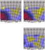 |
Fig.C.2
Upper panel: simulated synchrotron component (left) and synchrotron template (right) at 23 GHz. Lower panel: difference map divided by the simulated component. |
| Open with DEXTER | |
The simulated data-sets described above were analysed with the CCA method using the same procedure as applied to the real data; the results of this assessment are presented in Sect. 4.1. As a separate test, we verified the impact of the CMB component on the results for νp and m60. We generated 100 sets of mock data with the same foreground emission and different realizations of CMB and instrumental noise, and repeated the estimation of the AME frequency scaling. For this test we used the simulation with a spatially constant AME spectrum peaking at 26 GHz. As this analysis is computationally demanding, the CCA estimation was performed only on the ten independent patches covering the Gould Belt region (centred on latitudes −20° and −40° and longitudes of 140°, 160°, 180°, 200°, and 220°). In Fig. C.3 we show the average (diamonds) and rms (error bars) νp and m60 over the 100 realizations for each
patch for different patches on the x-axis. The scatter between the results obtained for different patches (indicated by the grey area in the plots) is typically larger than the error bars, measuring the scatter due to different CMB realizations. This means that the foreground emission generally dominates over the CMB as a source of error. Larger error bars associated with the CMB are obtained for three patches with faint foreground emission. For these patches the estimated errors on νp and m60 are consistently larger. The CMB variation results on average in Δνp = 0.1 GHz and Δm60 = 0.3, which reach 0.3 GHz and 0.8, respectively, for the poorest sky patch. These values are below the error bars resulting from the analysis of the data, which amount to 1–1.5 GHz for νp and 1.5–2 for m60. The CMB has limited impact on the results because this component is modelled in the mixing matrix. Having a known frequency scaling, the statistical constraint used by CCA is able to trace the pattern of the CMB through the frequencies with good precision and hence identify it correctly.
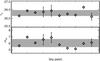 |
Fig.C.3
Average and rms of νp and m60 estimated over simulations with different CMB and noise realizations for different patches on the x-axis. The grey area is the average and rms over different patches, which is typically larger than that due to noise and CMB. |
| Open with DEXTER | |
© ESO, 2013
Current usage metrics show cumulative count of Article Views (full-text article views including HTML views, PDF and ePub downloads, according to the available data) and Abstracts Views on Vision4Press platform.
Data correspond to usage on the plateform after 2015. The current usage metrics is available 48-96 hours after online publication and is updated daily on week days.
Initial download of the metrics may take a while.