| Issue |
A&A
Volume 555, July 2013
|
|
|---|---|---|
| Article Number | A96 | |
| Number of page(s) | 8 | |
| Section | Stellar structure and evolution | |
| DOI | https://doi.org/10.1051/0004-6361/201220622 | |
| Published online | 08 July 2013 | |
Online material
Appendix A: Codes and input physics
The BaSTI code for white dwarf evolutionary calculations solves the four equations describing the structure of a star by applying a Raphson-Newton method, following the techniques described in, e.g., Kippenhahn et al. (2013). The independent variable is the mass Mr and the independent variables are radius (r), pressure (P), luminosity (l), and temperature (T). The model structure is divided into an interior and an exterior layer whose thickness can be chosen. In our calculations we fixed the mass fraction of this exterior layer to q = 10-6, two orders of magnitude smaller than the thickness of the hydrogen envelope. This extremely thin layer is modelled by integrating the equations dR/dP, dM/dP, and dT/dP, with P as the independent variable, considering the luminosity l constant, by means of a fourth-order Runge-Kutta method. The starting point is the bottom of the atmosphere, whose pressure is provided either by an Eddington T(τ) integration, or from detailed non-grey model atmospheres (see Salaris et al. 2010). This integration provides the outer boundary for the Newton-Raphson integration of the full set of equations with a centred scheme, to model the rest of the star. In these white dwarf calculations the mass distribution of the mesh points has been set by the requirement that R, l, P, T, and M do not vary by more than a fixed amount from one mesh point to the next at the beginning of the calculations. The total number of mesh points in the models discussed here is ~1000. The time step is set by the requirement that R, l, P, and T do not vary from one model to the next at each mesh point by more than δR/R = 0.01, δl/l = 0.02, δP/P = 0.05, and δT/T = 0.05.
The standard input physics for the carbon-oxygen core includes the EOS of Straniero (1988) in the gaseous phase, while for the liquid and solid phases the detailed EOS of Segretain et al. (1994) is used. As for the envelope H and He regions, the results of Saumon et al. (1995) are employed, supplemented at the highest densities by an EOS for H and He using the prescriptions of Segretain et al. (1994). Crystallization is considered to occur at Γ = 180, where Γ is the plasma ion coupling parameter. The associated release of latent heat is assumed to be equal to 0.77kBT per ion (kB denoting the Boltzmann constant).
The additional energy release due to phase separation of the carbon-oxygen mixture upon crystallization is computed following Isern et al. (1997, 2000). Neutrino energy losses are from Itoh et al. (1996) and Haft et al. (1994) for plasma-neutrino emission. The conductive opacities of Itoh et al. (1983) and Mitake et al. (1984) for the liquid and solid phases are adopted. For the range of temperatures and densities not covered by the previous results, the conductivities by Hubbard & Lampe (1969) are instead used. OPAL radiative opacities (Iglesias & Rogers 1996) with Z = 0 are used for T > 6000 K in the He and H envelopes. In the H envelope, and for the temperatures and densities not covered by the OPAL tables, Rosseland mean opacities come from the monochromatic opacities of Saumon & Jacobson (1999). Equation of state and opacity tables for various carbon-oxygen ratios are employed, and the interpolation in chemical composition is linear in the carbon abundance. At fixed chemical composition the opacity interpolation is cubic in log T and log ρ, whilst the EOS interpolation is linear in log T and log P. Convection is treated with the standard mixing-length formalism by Böhm-Vitense (1958) with mixing length α = 1.5.
The stellar evolution code LPCODE is based on the same standard method to solve the stellar structure equations. Three envelope integrations from the photosphere inward to a fitting outer mass fraction (q = 10-10) are performed to specify the outer boundary conditions. The independent variable is ξ = ln(1 − Mr/M∗) and the dependent variables are R, P, l, and T. A change of variables is considered in LPCODE:
with uθ, up, ux, and ul being the quantities to be iterated that are given by uθ = ΔT/T(n), up = ΔP/P(n), ux = ΔR/R(n), and ul = l, where superscripts n and n + 1 denote the beginning and end of time interval. Here, θ = ln T, x = ln R, and p = ln P. Thus, the Newton-Raphson iteration scheme is applied to the differences in the luminosity, pressure, temperature, and radius between the previous and the computed model. For the white dwarf regime, a centred scheme is used for the equations of stellar structure and evolution. Models are divided into approximately 1000–1500 mesh points.
The LPCODE employs the EOS of Segretain et al. (1994) for the high-density regime (above a density of 8 × 10² g/cm3) complemented with an updated version of the EOS of Magni & Mazzitelli (1979) for the low-density regime. Radiative opacities above 11 000 K and neutrino energy losses are as in the BaSTI code, while for temperatures below 8000 K radiative opacities from the AESOPUS database (Marigo & Aringer 2009) are employed, and in the intermediate regime an interpolation between OPAL and AESOPUS opacities is performed; OPAL radiative opacities are calculated directly from the interpolation routine provided by OPAL (version: Arnold Boothroyd, April 27, 2001). Arbitrary hydrogen abundances and arbitrary amounts of excess carbon and oxygen are always allowed. In this paper, Z = 0 is considered. The routine performs interpolations up to 6 variables to get the opacity at the given composition, temperature, and density.
Electron conduction opacities are taken from Cassisi et al. (2007). Neutrino energy losses, the release of latent heat and carbon-oxygen phase separation upon crystallization are treated in the same way as in the BaSTI code. Latent heat is included self-consistenly and locally coupled to the full set of equations of stellar evolution, and is calculated at each iteration during the convergence of the model. The contribution is distributed over a small mass range around the crystallization front. Outer boundary conditions are derived from non-grey model atmospheres (Rohrmann et al. 2012), or alternatively, from a standard Eddington T(τ) relation. Convection is treated with the standard Böhm-Vitense (1958) mixing length formalism and mixing length α = 1.61.
Appendix A: The role of electron conduction opacities
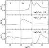 |
Fig. A.1
Relative difference of the stellar opacity Δk/k as a function of gas pressure, at fixed T, ρ, and chemical stratifications taken from three models calculated with the BaSTI code at step 2, with the labelled luminosities (see text for details). The H, He, and C regions, as well as the lower boundary of surface convection, are marked. |
| Open with DEXTER | |
As mentioned in our comparison of carbon core models, the relevant regions where the choice of the conduction opacities makes a difference are the carbon core at high luminosities (above log (L/L⊙) ~ −2), the helium envelope at intermediate luminosites (between log (L/L⊙) ~ −2 and log (L/L⊙) ~ −4.0), and the hydrogen envelope at low luminosities (below log (L/L⊙) ~ −4.0). Figure A.1 displays the difference of the total opacity at fixed T, ρ, and chemical stratifications (from the BaSTI calculations at step 2) for three different luminosities. The difference is between the values obtained employing the Cassisi et al. (2007) conduction opacities, minus the results obtained from the combination of Itoh et al. (1983), Mitake et al. (1984), and Hubbard & Lampe (1969) conduction opacities used as standard input in BaSTI calculations. As shown by Fig. A.1, in the high luminosity regime electron conduction opacities by Cassisi et al. (2007) are higher mainly in the carbon core, and this turns out to
increase the neutrino energy losses, causing a faster cooling. This connection between increased opacities in the core of bright, hot models, and increased neutrino emission has been verified by a numerical experiment, where we have calculated a cooling sequence by artifically enhancing the opacity of the carbon core at high luminosities.
At intermediate luminosities it is the opacity of the helium layers that increases when employing Cassisi et al. (2007) results. In this case the effect is a slowing down of the cooling due to the higher opacity of the helium envelope. At low luminosities it is instead the higher opacity of the degenerate hydrogen layers that has a major effect on the cooling speed. We also find large variations of the carbon core opacity (see Fig. A.1) that are, however, irrelevant in this regime, because the opacity of the core is extremely small because of the high degree of degeneracy of the core. The effect of an increased opacity of the hydrogen layers at low luminosity actually speeds-up the cooling, as we have confirmed with a numerical experiment where we have computed a model by artificially enhancing the opacity of the degenerate layers of the hydrogen envelope. The reason for this counterintuitive result is the slightly deeper extension of the hydrogen convective envelope in this luminosity regime. After convective coupling has been established, at log (L/L⊙) ~ −4.0 in these models, the cooling becomes faster compared to the case of no coupling because of a more efficient energy transport. The energy transport efficiency is increased when convection extends deeper into the degenerate hydrogen layers, thus increasing the cooling speed as well. These three effects explain the difference between the Δt/t values determined at steps 1 and 2 of our pure carbon core model comparisons.
© ESO, 2013
Current usage metrics show cumulative count of Article Views (full-text article views including HTML views, PDF and ePub downloads, according to the available data) and Abstracts Views on Vision4Press platform.
Data correspond to usage on the plateform after 2015. The current usage metrics is available 48-96 hours after online publication and is updated daily on week days.
Initial download of the metrics may take a while.