| Issue |
A&A
Volume 555, July 2013
|
|
|---|---|---|
| Article Number | A96 | |
| Number of page(s) | 8 | |
| Section | Stellar structure and evolution | |
| DOI | https://doi.org/10.1051/0004-6361/201220622 | |
| Published online | 08 July 2013 | |
Research Note
Comparison of theoretical white dwarf cooling timescales⋆,⋆⋆
1
Astrophysics Research Institute, Liverpool John Moores
University, Liverpool Science Park, IC2 Building,
146 Brownlow
Hill
Liverpool
L3 5RF
UK
e-mail:
This email address is being protected from spambots. You need JavaScript enabled to view it.
2
Grupo de Evolución Estelar y Pulsaciones, Facultad de Ciencias
Astronómicas y Geofísicas, Universidad Nacional de La Plata,
Paseo del Bosque s/n,
1900
La Plata,
Argentina
3
CCT La Plata, CONICET, 1900
La Plata,
Argentina
e-mail:
This email address is being protected from spambots. You need JavaScript enabled to view it.
4
Departament de Física Aplicada, Universitat Politècnica de
Catalunya, c/Esteve Terrades
5, 08860
Castelldefels,
Spain
e-mail:
This email address is being protected from spambots. You need JavaScript enabled to view it.
5
Institute for Space Studies of Catalonia,
c/Gran Capità 2–4, Edif. Nexus
104, 08034
Barcelona,
Spain
Received: 24 October 2012
Accepted: 29 May 2013
Abstract
Context. An accurate assessment of white dwarf cooling times is paramount so that white dwarf cosmochronology of Galactic populations can be put on more solid grounds. This issue is particularly relevant in view of the enhanced observational capabilities provided by the next generation of extremely large telescopes, that will offer more avenues to use white dwarfs as probes of Galactic evolution and test-beds of fundamental physics.
Aims. We estimate for the first time the consistency of results obtained from independent evolutionary codes for white dwarf models with fixed mass and chemical stratification, when the same input physics is employed in the calculations.
Methods. We compute and compare cooling times obtained from two independent and widely used stellar evolution codes, BaSTI and LPCODE evolutionary codes, using exactly the same input physics for 0.55 M⊙ white dwarf models with both pure carbon and uniform carbon-oxygen (50/50 mass fractions) cores, and pure hydrogen layers with mass fraction qH = 10-4MWD on top of pure helium buffers of mass qHe = 10-2MWD.
Results. Using the same radiative and conductive opacities, photospheric boundary conditions, neutrino energy loss rates, and equation of state, cooling times from the two codes agree within ~2% at all luminosities, except when log (L/L⊙) > −1.5 where differences up to ~8% do appear, because of the different thermal structures of the first white dwarf converged models at the beginning of the cooling sequence. This agreement is true for both pure carbon and uniform carbon-oxygen stratification core models, and also when the release of latent heat and carbon-oxygen phase separation are considered. We have also determined quantitatively and explained the effect of varying equation of state, low-temperature radiative opacities, and electron conduction opacities in our calculations,
Conclusions. We have assessed for the first time the maximum possible accuracy in the current estimates of white dwarf cooling times, resulting only from the different implementations of the stellar evolution equations and homogeneous input physics in two independent stellar evolution codes. This accuracy amounts to ~2% at luminosities lower than log (L/L⊙) ~ −1.5. This difference is smaller than the uncertainties in cooling times attributable to the present uncertainties in the white dwarf chemical stratification. Finally, we extend the scope of our work by providing tabulations of our cooling sequences and the required input physics that can be used as a comparison test of cooling times obtained from other white dwarf evolutionary codes.
Key words: stars: interiors / stars: evolution / white dwarfs
Tables 1 to 4, the equation of state, boundary conditions, and CO phase diagram routines are only available at the CDS via anonymous ftp to cdsarc.u-strasbg.fr (130.79.128.5) or via http://cdsarc.u-strasbg.fr/viz-bin/qcat?J/A+A/555/A96
Appendices A and B are available in electronic form at http://www.aanda.org
© ESO, 2013
1. Introduction
During the last two decades white dwarf observations and theory have improved to a level that has finally made it possible to start employing white dwarfs as credible astrophysical tools (see Althaus et al. 2010a, for a recent review). A detailed assessment of the accuracy of current estimates of white dwarf cooling rates is therefore a pressing necessity, for carbon-oxygen white dwarfs are increasingly being employed to constrain the age and past history of Galactic populations, including the solar neighbourhood, open and globular clusters (see, i.e., Winget et al. 1987, 2009; García-Berro et al. 1988, 2010; Hansen et al. 2007; Bedin et al. 2008, 2010, and references therein). Furthermore, theoretical estimates of white dwarf cooling rates are routinely adopted to place constraints on the properties of neutrinos, exotic particles, and dark matter candidates (Freese 1984; Isern et al. 1992, 2008; Winget et al. 2004; Bertone & Fairbairn 2008; Córsico et al. 2012) and alternative theories of gravity (see, e.g., Garcia-Berro et al. 1995, 2011; Benvenuto et al. 2004). These types of investigations all demand an accurate calculation of white dwarf cooling models. This, in turn, requires a detailed and accurate knowledge of the main physical processes that affect the evolution of white dwarfs, and the initial chemical stratification for a given value of the white dwarf mass.
There have been a few recent theoretical studies to assess the sensitivity of the predicted cooling times to uncertainties in the model core and envelope chemical stratification and electron conduction opacities, (Hansen 1999; Prada Moroni & Straniero 2007; Salaris 2009; Salaris et al. 2010), and photospheric boundary conditions (Hansen 1999; Salaris et al. 2000; Rohrmann et al. 2012). However, there is no modern systematic study of the effect of employing different equations of state (EOS) and radiative opacities, especially the less established low-temperature opacities in cool white dwarfs. Besides these potential sources of uncertainties, there is an even more pressing need to assess the consistency of results obtained from independent evolutionary codes for white dwarf models with a fixed mass, adopting the same input physics and chemical stratification. Differences determined from this class of comparisons represent the maximum possible accuracy in the current estimates of white dwarf cooling times, determined only by the different implementations of the stellar evolution equations and input physics. Assessing the consistency of results of independent white dwarf stellar codes becomes absolutely necessary to place white dwarf cosmochronology on solid ground. This is even more important when considering that the next generation of extremely large telescopes, i.e., the European-Extremely Large Telescope (E-ELT), the Thirty Meter Telescope (TMT) and the Giant Magellan Telescope (GMT), and the new generation of astrometric satellites, Gaia for example, will open new avenues to exploit the potential of white dwarfs as probes of Galactic evolution and fundamental physics (see, i.e., Bono et al. 2013; Torres et al. 2005). Self-consistent comparisons of this type have never been performed. Similar tests discussed previously in the literature (Winget & van Horn 1987; Hansen & Phinney 1998) are not completely consistent, in the sense that the different codes compared were not employing exactly the same input physics, even though in one case (Winget & van Horn 1987) the effect of the different input physics adopted in the models available at the time was estimated, to reduce all calculations to approximately to the same physics setup.
For these reasons, we present here the first fully self-consistent comparison of cooling times obtained using exactly the same input physics from two independent evolutionary codes whose white dwarf calculations have been widely employed in the literature: The LPCODE evolutionary code (see Althaus et al. 2010b; Renedo et al. 2010, for recent references) and the BaSTI evolutionary code (see Salaris et al. 2010, and references therein). This is done for a white dwarf model with fixed chemical stratification. This approach is similar to the crucial tests performed in the field of asteroseismology (see, i.e., Marconi et al. 2008; Lebreton et al. 2008) where the same physics input is adopted to compare internal structure, evolution and seismic properties of stellar models. As a byproduct of these comparisons we also determine a rigorous estimate of the effect of varying the low-temperature radiative opacities, EOS, and electron conduction opacities amongst currently available tabulations.
To inspire other members of the white dwarf community to compare results from their evolutionary codes with this set of calculations (thus broadening the scope of this investigation by considering additional codes) we will make tables available with the results of our reference calculations discussed in the paper, and the physical ingredients adopted in these calculations that are not publicly available. This will be the first paper in a series aiming to assess comprehensively the uncertainties of white dwarf cosmochronology. It will be followed by an analysis of the effect of standard assumptions in the white dwarf calculations, like using – as customary – pure H and/or He buffers with chemical discontinuities at the boundaries vs. diffusive chemical transitions, and – relevant for bright white dwarfs, as demonstrated in this paper – comparison of models evolved through the thermally pulsing phase with models started artificially at the top of the cooling sequence. The final paper will try to establish the current most accurate physics inputs (e.g., EOS, boundary conditions, and opacities) for white dwarf evolutionary calculations. The outline of this paper is as follows. Section 2 describes briefly the codes and their standard assumptions about input physics, while Sect. 3 presents comparisons of cooling times by altering the model physics step-by-step until all inputs are the same in both sets of calculations. Conclusions close the paper.
2. Calculations and comparisons
Details about the input physics and numerical solution of the stellar structure equations in the BaSTI code and LPCODE, mesh distribution of the models, opacity, and EOS tables interpolations are given in the Appendix. We calculated two sets of cooling models, both for a white dwarf with a total mass M = 0.55 M⊙, and an envelope consisting of a pure H layer with mass fraction qH = 10-4MWD on top of a pure He layer of mass qHe = 10-2MWD . The first group of calculations envisages a pure carbon core. As a first baseline set we employed the standard input physics choices of the two codes, the Eddington T(τ) relation for the photospheric boundary condition and, to isolate the effect of just basic input physics, no latent heat release upon crystallization was considered. The different choices of physics inputs in the two codes are the low temperature opacities (below 8000 K), electron conduction opacities, and EOS (see Appendix).
The origin of the cooling age is set to zero at log (L/L⊙) = 1.1 in all calculations discussed in this paper and cooling times for these calculations are compared in Fig. 1. This diagram displays the relative age difference Δt = (tBaSTI − tLPCODE)/tBaSTI as a function of the luminosity of the white dwarf. Ages from the BaSTI model are also marked at representative luminosities1. As can be observed, BaSTI ages appear typically larger at luminosities above log (L/L⊙) ~ −2.0, and smaller at lower luminosities, apart from the spike at log (L/L⊙) ~ −4.2. In spite of some different physics inputs in the two codes, age differences are within about ±10% at fixed luminosity.
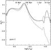 |
Fig. 1 Relative age difference Δt/t = (tBaSTI − tLPCODE)/tBaSTI as a function of the luminosity for the 0.55 M⊙ carbon-core sequence. The case with the standard input physics of the two codes (detailed in Sect. 2) is displayed as a solid line. No latent heat release upon crystallization is included, and an Eddington T(τ) relation is employed for the outer boundary conditions. Selected ages from the BaSTI model are also marked at representative luminosities. Dash-dotted and dashed lines display additional comparisons by changing the EOS in the model calculations (see text for details). |
We then proceeded to calculate additional sets of pure carbon models (still no latent heat release at crystallization) changing the inconsistent physics input one at a time according to the following steps:
-
1.
Calculations with both the BaSTI and the LPCODE evolutionarycodes employing the Magni & Mazzitelli (1979)EOS everywhere, that is, in both the core and the envelope. We usehere exactly the same EOS numerical routine in both codes. Weuse this EOS because the routine is easy to implement and coversthe entire structure of the white dwarf, thus simplifying thereplacement of the standard EOS choices in both codes.Comparisons of cooling times at this step cancel the effect of usinga different EOS in the two calculations.
-
2.
Calculation of BaSTI models with the previously mentioned EOS and electron conduction opacities by Cassisi et al. (2007), as in the LPCODE calculations. The same numerical routine to calculate the electron conduction opacities is used, but the two codes employ different sets of total (radiative plus conduction) opacity tables and different interpolation schemes. Comparisons of BaSTI model cooling times at this step with LPCODE results at the previous step cancel the effect of the difference in the conduction opacities between the two calculations.
-
3.
Calculations of both LPCODE and BaSTI models with the EOS of Magni & Mazzitelli (1979), electron conduction opacities by Cassisi et al. (2007), employing now photospheric boundary conditions taken at an optical depth τ = 25 from the model atmospheres by Rohrmann et al. (2012) when Teff < 10 000 K 2. The same table of photospheric boundary conditions is used in both calculations. Comparisons of cooling times at this step cancel the remaining effect of using different low temperature opacities in the two calculations because in cool white dwarf models and at the optical depths where the boundary condition is fixed, the envelope is convective and largely adiabatic. This makes a detailed knowledge of the low-temperature radiative opacity much less relevant.
The results of the comparisons at step 1 (displayed as a dash-dotted line), 2 (dashed line) and 3 (solid line) are shown in Fig. 2. We discuss first the effect of changing the EOS by recalling that in the standard input physics case BaSTI and LPCODE models share the same EOS at high densities, but employe a different EOS in the low-density regime. To this purpose, in addition to the relative age differences obtained with the standard input physics of the two codes (solid line), Fig. 1 also displays Δt/t for the input physics at step 1 (dash-dotted line, as shown also in Fig. 2) and the age difference between the BaSTI calculations at step 1 and the LPCODE calculations with standard physics (short-dashed line). A comparison of the solid and short-dashed lines that display Δt/t with respect to the same reference cooling track, shows how, starting from log (L/L⊙) ~ −2.0, the Magni & Mazzitelli (1979) EOS causes increasingly and substantially shorter cooling timescales compared to the use of the EOS by Segretain et al. (1994) at high densities, and by Saumon et al. (1995) in the envelope. The main reason for these differences is the lower value of the specific heat for the carbon core that reaches differences of ~40–50% at the centre of the faintest models. If we now consider the dash-dotted line that shows the comparison with the input physics of step 1, e.g., with the same Magni & Mazzitelli (1979) EOS everywhere in both sets of calculations, Δt/t moves back to be very close to the case with standard physics.
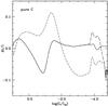 |
Fig. 2 Relative age difference Δt/t = (tBaSTI − tLPCODE)/tBaSTI as a function of luminosity for carbon-core sequences. No latent heat release upon crystallization is assumed. Dash-dotted line, dashed line, and solid line correspond to different input physics as specified at steps 1, 2, and 3 in the text. In particular, at step 3 the input physics assumed in both codes is exactly the same (see text for details). |
By recalling that for the standard case (solid line) the EOS employed in the two sets of models was different only in the low-density regime, and that at step 1 (dash-dotted line) it is the same everywhere, the comparison of Δt/t for these two cases suggests that the difference between Saumon et al. (1995) and Magni & Mazzitelli (1979) EOS at low-densities, e.g., differences of the specific heat increasing with decreasing luminosities up to ~±50%, and smaller differences of the adiabatic gradient of the order of ~±10–20%, has a very small effect on the cooling times, at least down to log (L/L⊙) ~ −4.0. At these low luminosities it is the onset of convective coupling (D’Antona & Mazzitelli 1990; Fontaine et al. 2001) that causes the different behaviour of Δt/t between the two cases. Convective coupling occurs when the base of the convective envelope reaches into degenerate layers (within the hydrogen envelope) coupling the surface with the degenerate interior, and increasing the rate of energy transfer across the envelope. When convective coupling sets in, the envelope becomes significantly more transparent and there is initially an excess of thermal energy that the star must radiate away. The release of this excess energy delays the cooling process for a while. Because of the slightly lower adiabatic gradient in the hydrogen layers obtained from the Saumon et al. (1995) EOS (differences ~10% in the deeper hydrogen layers), the convective envelope is more extended, and convective coupling sets in earlier compared to calculations with the Magni & Mazzitelli (1979) EOS in the envelope. This explains the bump in Δt/t seen around log (L/L⊙) ~ −4.2 for the comparison with the standard imputs; the bump disappears in the comparison at step 1 (compare the dash-dotted with the solid line in Fig. 1) when the same EOS is employed everywhere. Overall, when the two sets of calculations employ the same EOS for the whole structures, there are still differences of ±10% in the cooling times. Now, BaSTI models cool systematically more quickly than LPCODE ones below log (L/L⊙) ~ −2.0, and more slowly at higher luminosities.
Employing the same electron conduction opacities (dashed line in Fig. 2 that overlaps with the solid line at luminosities above log (L/L⊙) ~ −3.5) makes the cooling times much closer, highlighting the major role played by the different electron conduction tables employed in the two codes. The relevant regions (within the models) where the choice of the conduction opacities makes a difference are the carbon core at high luminosities (above log (L/L⊙) ~ −2), the helium envelope at intermediate luminosites (between log (L/L⊙) ~ −2 and log (L/L⊙) ~ −4.0), and the hydrogen envelope at low luminosities (below log (L/L⊙) ~ −4.0). The details of the opacity differences and their impact on the cooling timescales are discussed in the Appendix.
After step 2 the larger disagreement is now circumscribed at luminosities above log (L/L⊙) ~ −1.5, where the sign of Δt is reversed compared to the previous step, and below log (L/L⊙) ~ −3.5. This latter discrepancy vanishes once boundary conditions from the same model atmosphere calculations are employed in both BaSTI and LPCODEmodels (solid line). As mentioned before, in this case we are circumventing the difference of low-temperature opacities adopted in the two codes. It is also important to notice that when boundary conditions from model atmospheres are employed and matched at our chosen optical depth τ = 25, the underlying convective envelope (when convection is present) is always adiabatic. The superadiabatic layers are located at lower optical depths, and the white dwarf model becomes insensitive to the choice of the mixing length value in the stellar evolution calculations. In this case the superadiabatic layers are included in the model atmosphere calculations, and the superadiabatic convection treatment will affect the evolutionary model indirectly through the surface boundary condition. From this point of view, very recent advances in 3D radiation hydrodynamics white dwarf model atmosphere calculations (Tremblay et al. 2013) hold the promise of finally eliminating the uncertainty in the cooling evolution attributable to the treatment of superadiabatic convection.
At the end of this final step, when the input physics is exactly the same in both codes, cooling times agree within ~2% everywhere, but in the region above log (L/L⊙) ~ −1.5 (absolute ages of the order of ~10 Myr or less), where differences up to ~8% do still appear. As we will discuss later, this discrepancy is due to the different physical conditions of the first model converged at the beginning of the cooling sequence that are erased by the end of the early phase (first ≈108 yr of cooling) of efficient neutrino energy losses (the so-called neutrino cooling phase). We want to mention that these discrepancies at high luminosities still remain, even when we use exactly the same numerical routine to compute neutrino emission rates.
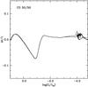 |
Fig. 3 Relative age difference Δt/t = (t(BaSTI) − tLPCODE)/tBaSTI as a function of luminosity for sequences with cores made of a 50/50 carbon-oxygen mixture. The input physics in both codes is exactly the same, as specified at step 3 for the pure carbon sequences. Dash-dotted, dashed, and solid lines correspond to calculations without latent heat and phase separation, with latent heat and no phase separation, and with both latent heat and phase separation, respectively. |
A second group of cooling models for a white dwarf with the same mass and envelope stratification, but now with a 50/50 carbon-oxygen core composition (by mass), were then calculated with both codes using consistent input physics as at step 3 of the pure carbon models. The purpose of this group of calculations is to compare results with a mixed carbon-oxygen core composition and also with the inclusion of latent heat release (we adopt 0.77kBT per crystallized ion in both codes) and phase separation upon crystallization. The test proceeded in three steps3:
-
1.
Calculations without release of latent heat and phaseseparation.
-
2.
Calculations with latent heat release but without phase separation.
-
3.
Calculations with both latent heat release and phase separation.
Both codes include phase separation by considering in the release of energy per gram of crystallized matter an extra term given by Eq. (2) in Isern et al. (2000), namely ![Mathematical equation: \begin{equation} \epsilon_{\rm g}=-\Delta X_0 \left[\left(\frac{\partial E}{\partial X_0}\right)_{M_{\rm s}}- \left\langle\frac{\partial E}{\partial X_0}\right\rangle\right] \end{equation}](/articles/aa/full_html/2013/07/aa20622-12/aa20622-12-eq33.png) (1)where
(1)where  is the difference of oxygen abundance between the solid and liquid phase in the crystallizing layer (we employed the Segretain & Chabrier 1993, carbon-oxygen diagram in both codes) and E is the internal energy per unit mass. The first term represents the energy released in the layer that is crystallizing, because of the increase of the oxygen abundance caused by phase separation, whereas the second term represents the average amount of energy absorbed in the convective layers that appear just above the crystallization front as a consequence of the local decrease of the oxygen abundance. The derivative (∂E/∂X0)V,T is determined layer-by-layer employing Eqs. (6) and (7) in Isern et al. (2000).
The results of the comparisons at steps 1, 2, and 3 are shown in Fig. 3. The cooling age differences between BaSTI and LPCODE models obtained for these three different steps overlap at luminosities brighter than log (L/L⊙) ~ −4.0 that marks the onset of crystallization. In quantitative terms, at luminosities above log (L/L⊙) ~ −1.5 relative differences are slightly smaller than in the case of pure carbon models, but are still appreciable, again because of differences in the initial model at the start of the cooling sequence. At lower luminosities, relative age differences are essentially the same as in the case of the pure carbon models with consistent input physics. The inclusion of the release of latent heat in these calculations and of phase separation do not substantially alter the quantitative result. There are some oscillations or spikes in the behaviour of Δt with luminosity during the crystallization of the core, that can be ascribed to the different numerical implementation of the latent heat and energy release due to phase separation. Both codes, for reasons of numerical stability, distribute this energy release over a narrow mass interval around the crystallization front, and the different implementations of this mechanism cause the narrow spikes seen in Δt at low luminosities. On the whole, relative age differences are again very small, within ~2% at luminosities below log (L/L⊙) ~ −1.5.
The relative differences of the total radius R are within 0.5% and differences in central temperature Tc are within 1% for luminosities below log (L/L⊙) ~ −1.5 (BaSTI models displaying larger R and Tc) independent of the inclusion of the release of latent heat and/or phase separation. Differences in both radius and central temperature increase steadily towards higher luminosities, reaching ~20% in Tc and ~3% in R at log (L/L⊙) ~ 1.0. This is another consequence of the different thermal stratification of the structures at the top of the cooling sequence, with the BaSTI models initially hotter and less degenerate in the central regions. Only at the end of the neutrino cooling phase do both Tc and R converge to approximately the same values in the two calculations. Figure 4 compares the stratification of the temperature and density in the core of two BaSTI models with luminosities equal to, respectively, log (L/L⊙) = 1.03 and 0.82, and a LPCODE model with log (L/L⊙) = 0.96. These models correspond to the 0.55 M⊙ carbon-oxygen calculations with the same input physics in both codes. In principle, if the BaSTI and LPCODE initial models were identical, the structure of the LPCODE model in Fig. 4 should lie between the two BaSTI results, because its surface luminosity is intermediate between the two BaSTI models. Instead, the inner part of the core (when log ρ > 5.6) of both BaSTI models is hotter than the LPCODE model, a consequence of the higher temperatures in the core of the first structure at the top of the cooling sequence. This is an important reminder that when sets of white dwarf models are calculated by artificially starting the cooling sequence with pre-determined carbon-oxygen and envelope stratifications (i.e., not derived from the full progenitor evolution), the technical details of how the first white dwarf model is built, can induce appreciable differences in the evolution before the end of the neutrino cooling phase. Our comparison provides an order-of-magnitude estimate of these uncertainties for the first time.
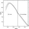 |
Fig. 4 Temperature-density stratification in two BaSTI models (dashed lines) and one LPCODE model (solid line) at the top of the cooling track for the sequence in which a 50/50 carbon-oxygen mixture is adopted. See text for details. |
3. Conclusions
We have performed the first consistent comparison of white dwarf cooling times determined from two widely used, independent stellar evolution codes (BaSTI and LPCODE) employing exactly the same input physics. Cooling age differences determined from these comparisons represent the maximum possible accuracy in the current estimates of white dwarf cooling times, arising only from the different implementations of the stellar evolution equations and input physics.
We first considered a 0.55 M⊙ model with a pure carbon core, and pure hydrogen layers with mass fraction qH = 10-4MWD on top of a pure helium buffer of mass qHe = 10-2MWD. At this stage, latent heat release upon crystallization was neglected. When the same OPAL radiative opacities and Cassisi et al. (2007) electron conduction opacities, photospheric boundary conditions from the model atmospheres by Rohrmann et al. (2012), neutrino energy loss rates (Itoh et al. 1996; Haft et al. 1994), and EOS (Magni & Mazzitelli 1979) are employed, cooling times obtained from the two codes agree within ~2% at all luminosities, with the exclusion of models brighter than log (L/L⊙) ~ −1.5, where differences up to ~8% appear because of the different thermal structure of the first white dwarf structure converged at the beginning of the cooling sequence.
We then considered a 0.55 M⊙ model with a uniform carbon-oxygen stratification (50/50 by mass) in the core, and the same hydrogen and helium envelope. We calculated models with the same input physics listed above, without taking into account the release of latent heat and disregarding phase separation during crystallization, including only the release of latent heat, and finally considering both contributions, using the phase diagram of Segretain & Chabrier (1993) and the treatment of Isern et al. (1997, 2000) for the energy release due to phase separation. Relative age differences are always very small, within ~2% at luminosities below log (L/L⊙) ~ −1.5. This 2% difference is smaller than the current uncertainties in cooling times because of uncertainties in the white dwarf chemical stratification (see, e.g., Salaris et al. 2010). At higher luminosities differences up to ~8% are found again, due to differences in the thermal stratification of the starting model.
As already mentioned in the introduction, to broaden the scope of this study by facilitating comparisons with additional codes employed by the white dwarf community, we provide tables with the BaSTI cooling tracks for the three carbon-oxygen sequences with and without considering the release of latent heat and/or considering phase separation, and the sequence with a carbon core without release of latent heat, all calculated with the input physics listed above. We also provide the routine for the EOS of Magni & Mazzitelli (1979) and the phase diagram of Segretain & Chabrier (1993) as tabulated in our codes. All other physics ingredients are publicly available and most of them widely used in modern white dwarf calculations.
Before closing, we wish to restate that the goal of this study is to compare results from independent white dwarf cooling codes when using the same input physics, not to provide up-to-date white dwarf models to compare with observations. Specifically, and for ease of implementation, we use in our common physics inputs the EOS of Magni & Mazzitelli (1979), which is a simplification of the EOS implemented in our respective codes. As already mentioned in the previous section, switching from this EOS to that of Saumon et al. (1995) in the hydrogen-helium envelopes provides the same cooling times within ~1% at luminosities brighter than the onset of convective coupling. However, the situation is different for the core, as already discussed on the basis of a comparison of the specific heat in the pure carbon models. As an additional test using the LPCODE, we performed calculations switching from the EOS of Magni & Mazzitelli (1979) to that of Segretain et al. (1994) in a model with pure carbon core, the model at step 3 of the carbon core comparisons in the previous section. Cooling times are reduced by up to ~20–30%, mainly during the crystallization phase, when the EOS of Magni & Mazzitelli (1979) is employed, consistent with the results shown in Fig. 1. It is therefore clear that this EOS provides sizably shorter cooling times compared to more modern EOS calculations when employed in the degenerate carbon-oxygen cores (but this EOS is still accurate for the hydrogen and helium envelopes). However, given that what matters here is the difference of cooling times predicted by independent evolutionary codes for a fixed set of input physics, a potential inadequacy of the EOS of Magni & Mazzitelli (1979) compared to more modern EOS calculations is irrelevant in this context, and does not affect either the outcome or the validity of these tests.
Online material
Appendix A: Codes and input physics
The BaSTI code for white dwarf evolutionary calculations solves the four equations describing the structure of a star by applying a Raphson-Newton method, following the techniques described in, e.g., Kippenhahn et al. (2013). The independent variable is the mass Mr and the independent variables are radius (r), pressure (P), luminosity (l), and temperature (T). The model structure is divided into an interior and an exterior layer whose thickness can be chosen. In our calculations we fixed the mass fraction of this exterior layer to q = 10-6, two orders of magnitude smaller than the thickness of the hydrogen envelope. This extremely thin layer is modelled by integrating the equations dR/dP, dM/dP, and dT/dP, with P as the independent variable, considering the luminosity l constant, by means of a fourth-order Runge-Kutta method. The starting point is the bottom of the atmosphere, whose pressure is provided either by an Eddington T(τ) integration, or from detailed non-grey model atmospheres (see Salaris et al. 2010). This integration provides the outer boundary for the Newton-Raphson integration of the full set of equations with a centred scheme, to model the rest of the star. In these white dwarf calculations the mass distribution of the mesh points has been set by the requirement that R, l, P, T, and M do not vary by more than a fixed amount from one mesh point to the next at the beginning of the calculations. The total number of mesh points in the models discussed here is ~1000. The time step is set by the requirement that R, l, P, and T do not vary from one model to the next at each mesh point by more than δR/R = 0.01, δl/l = 0.02, δP/P = 0.05, and δT/T = 0.05.
The standard input physics for the carbon-oxygen core includes the EOS of Straniero (1988) in the gaseous phase, while for the liquid and solid phases the detailed EOS of Segretain et al. (1994) is used. As for the envelope H and He regions, the results of Saumon et al. (1995) are employed, supplemented at the highest densities by an EOS for H and He using the prescriptions of Segretain et al. (1994). Crystallization is considered to occur at Γ = 180, where Γ is the plasma ion coupling parameter. The associated release of latent heat is assumed to be equal to 0.77kBT per ion (kB denoting the Boltzmann constant).
The additional energy release due to phase separation of the carbon-oxygen mixture upon crystallization is computed following Isern et al. (1997, 2000). Neutrino energy losses are from Itoh et al. (1996) and Haft et al. (1994) for plasma-neutrino emission. The conductive opacities of Itoh et al. (1983) and Mitake et al. (1984) for the liquid and solid phases are adopted. For the range of temperatures and densities not covered by the previous results, the conductivities by Hubbard & Lampe (1969) are instead used. OPAL radiative opacities (Iglesias & Rogers 1996) with Z = 0 are used for T > 6000 K in the He and H envelopes. In the H envelope, and for the temperatures and densities not covered by the OPAL tables, Rosseland mean opacities come from the monochromatic opacities of Saumon & Jacobson (1999). Equation of state and opacity tables for various carbon-oxygen ratios are employed, and the interpolation in chemical composition is linear in the carbon abundance. At fixed chemical composition the opacity interpolation is cubic in log T and log ρ, whilst the EOS interpolation is linear in log T and log P. Convection is treated with the standard mixing-length formalism by Böhm-Vitense (1958) with mixing length α = 1.5.
The stellar evolution code LPCODE is based on the same standard method to solve the stellar structure equations. Three envelope integrations from the photosphere inward to a fitting outer mass fraction (q = 10-10) are performed to specify the outer boundary conditions. The independent variable is ξ = ln(1 − Mr/M∗) and the dependent variables are R, P, l, and T. A change of variables is considered in LPCODE:
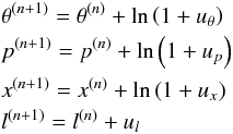 (A.1)
(A.1)
with uθ, up, ux, and ul being the quantities to be iterated that are given by uθ = ΔT/T(n), up = ΔP/P(n), ux = ΔR/R(n), and ul = l, where superscripts n and n + 1 denote the beginning and end of time interval. Here, θ = ln T, x = ln R, and p = ln P. Thus, the Newton-Raphson iteration scheme is applied to the differences in the luminosity, pressure, temperature, and radius between the previous and the computed model. For the white dwarf regime, a centred scheme is used for the equations of stellar structure and evolution. Models are divided into approximately 1000–1500 mesh points.
The LPCODE employs the EOS of Segretain et al. (1994) for the high-density regime (above a density of 8 × 10² g/cm3) complemented with an updated version of the EOS of Magni & Mazzitelli (1979) for the low-density regime. Radiative opacities above 11 000 K and neutrino energy losses are as in the BaSTI code, while for temperatures below 8000 K radiative opacities from the AESOPUS database (Marigo & Aringer 2009) are employed, and in the intermediate regime an interpolation between OPAL and AESOPUS opacities is performed; OPAL radiative opacities are calculated directly from the interpolation routine provided by OPAL (version: Arnold Boothroyd, April 27, 2001). Arbitrary hydrogen abundances and arbitrary amounts of excess carbon and oxygen are always allowed. In this paper, Z = 0 is considered. The routine performs interpolations up to 6 variables to get the opacity at the given composition, temperature, and density.
Electron conduction opacities are taken from Cassisi et al. (2007). Neutrino energy losses, the release of latent heat and carbon-oxygen phase separation upon crystallization are treated in the same way as in the BaSTI code. Latent heat is included self-consistenly and locally coupled to the full set of equations of stellar evolution, and is calculated at each iteration during the convergence of the model. The contribution is distributed over a small mass range around the crystallization front. Outer boundary conditions are derived from non-grey model atmospheres (Rohrmann et al. 2012), or alternatively, from a standard Eddington T(τ) relation. Convection is treated with the standard Böhm-Vitense (1958) mixing length formalism and mixing length α = 1.61.
Appendix A: The role of electron conduction opacities
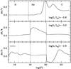 |
Fig. A.1 Relative difference of the stellar opacity Δk/k as a function of gas pressure, at fixed T, ρ, and chemical stratifications taken from three models calculated with the BaSTI code at step 2, with the labelled luminosities (see text for details). The H, He, and C regions, as well as the lower boundary of surface convection, are marked. |
As mentioned in our comparison of carbon core models, the relevant regions where the choice of the conduction opacities makes a difference are the carbon core at high luminosities (above log (L/L⊙) ~ −2), the helium envelope at intermediate luminosites (between log (L/L⊙) ~ −2 and log (L/L⊙) ~ −4.0), and the hydrogen envelope at low luminosities (below log (L/L⊙) ~ −4.0). Figure A.1 displays the difference of the total opacity at fixed T, ρ, and chemical stratifications (from the BaSTI calculations at step 2) for three different luminosities. The difference is between the values obtained employing the Cassisi et al. (2007) conduction opacities, minus the results obtained from the combination of Itoh et al. (1983), Mitake et al. (1984), and Hubbard & Lampe (1969) conduction opacities used as standard input in BaSTI calculations. As shown by Fig. A.1, in the high luminosity regime electron conduction opacities by Cassisi et al. (2007) are higher mainly in the carbon core, and this turns out to
increase the neutrino energy losses, causing a faster cooling. This connection between increased opacities in the core of bright, hot models, and increased neutrino emission has been verified by a numerical experiment, where we have calculated a cooling sequence by artifically enhancing the opacity of the carbon core at high luminosities.
At intermediate luminosities it is the opacity of the helium layers that increases when employing Cassisi et al. (2007) results. In this case the effect is a slowing down of the cooling due to the higher opacity of the helium envelope. At low luminosities it is instead the higher opacity of the degenerate hydrogen layers that has a major effect on the cooling speed. We also find large variations of the carbon core opacity (see Fig. A.1) that are, however, irrelevant in this regime, because the opacity of the core is extremely small because of the high degree of degeneracy of the core. The effect of an increased opacity of the hydrogen layers at low luminosity actually speeds-up the cooling, as we have confirmed with a numerical experiment where we have computed a model by artificially enhancing the opacity of the degenerate layers of the hydrogen envelope. The reason for this counterintuitive result is the slightly deeper extension of the hydrogen convective envelope in this luminosity regime. After convective coupling has been established, at log (L/L⊙) ~ −4.0 in these models, the cooling becomes faster compared to the case of no coupling because of a more efficient energy transport. The energy transport efficiency is increased when convection extends deeper into the degenerate hydrogen layers, thus increasing the cooling speed as well. These three effects explain the difference between the Δt/t values determined at steps 1 and 2 of our pure carbon core model comparisons.
The exact values of these ages will change in the additional calculations that follow, but the order of magnitude of the age at these selected luminosities will stay the same in all calculations discussed here.
The results of the BaSTI calculation are displayed in Table 1, available electronically at the CDS.
The results of the BaSTI calculations for each of these three steps are displayed in Tables 2–4, available electronically at the CDS.
Acknowledgments
We thank Marcelo Miller Bertolami for helpful discussions about some results from LPCODE calculations. Part of this work was supported by AGENCIA through the Programa de Modernización Tecnológica BID 1728/OC -AR, by PIP 112-200801-00940 grant from CONICET, by MCINN grant AYA2011–23102, by the ESF EUROCORES Program EuroGENESIS (MICINN grant EUI2009-04170), by the European Union FEDER funds, and by the AGAUR.
References
- Althaus, L. G., Córsico, A. H., Isern, J., & García-Berro, E. 2010a, A&ARv, 18, 471 [NASA ADS] [CrossRef] [Google Scholar]
- Althaus, L. G., García-Berro, E., Renedo, I., et al. 2010b, ApJ, 719, 612 [NASA ADS] [CrossRef] [Google Scholar]
- Bedin, L. R., King, I. R., Anderson, J., et al. 2008, ApJ, 678, 1279 [NASA ADS] [CrossRef] [Google Scholar]
- Bedin, L. R., Salaris, M., King, I. R., et al. 2010, ApJ, 708, L32 [NASA ADS] [CrossRef] [Google Scholar]
- Benvenuto, O. G., García-Berro, E., & Isern, J. 2004, Phys. Rev. D, 69, 082002 [NASA ADS] [CrossRef] [Google Scholar]
- Bertone, G., & Fairbairn, M. 2008, Phys. Rev. D, 77, 043515 [NASA ADS] [CrossRef] [Google Scholar]
- Böhm-Vitense, E. 1958, ZAp, 46, 108 [NASA ADS] [Google Scholar]
- Bono, G., Salaris, M., & Gilmozzi, R. 2013, A&A, 549, A102 [NASA ADS] [CrossRef] [EDP Sciences] [Google Scholar]
- Cassisi, S., Potekhin, A. Y., Pietrinferni, A., Catelan, M., & Salaris, M. 2007, ApJ, 661, 1094 [NASA ADS] [CrossRef] [Google Scholar]
- Córsico, A. H., Althaus, L. G., Miller Bertolami, M. M., et al. 2012, MNRAS, 424, 2792 [NASA ADS] [CrossRef] [Google Scholar]
- D’Antona, F., & Mazzitelli, I. 1990, ARA&A, 28, 139 [NASA ADS] [CrossRef] [Google Scholar]
- Fontaine, G., Brassard, P., & Bergeron, P. 2001, PASP, 113, 409 [NASA ADS] [CrossRef] [Google Scholar]
- Freese, K. 1984, ApJ, 286, 216 [NASA ADS] [CrossRef] [Google Scholar]
- García-Berro, E., Hernanz, M., Isern, J., & Mochkovitch, R. 1988, Nature, 333, 642 [NASA ADS] [CrossRef] [Google Scholar]
- Garcia-Berro, E., Hernanz, M., Isern, J., & Mochkovitch, R. 1995, MNRAS, 277, 801 [NASA ADS] [CrossRef] [Google Scholar]
- García-Berro, E., Torres, S., Althaus, L. G., et al. 2010, Nature, 465, 194 [NASA ADS] [CrossRef] [PubMed] [Google Scholar]
- García-Berro, E., Lorén-Aguilar, P., Torres, S., Althaus, L. G., & Isern, J. 2011, J. Cosmology Astropart. Phys., 5, 21 [Google Scholar]
- Haft, M., Raffelt, G., & Weiss, A. 1994, ApJ, 425, 222 [NASA ADS] [CrossRef] [Google Scholar]
- Hansen, B. M. S. 1999, ApJ, 520, 680 [NASA ADS] [CrossRef] [Google Scholar]
- Hansen, B. M. S., & Phinney, E. S. 1998, MNRAS, 294, 557 [NASA ADS] [CrossRef] [Google Scholar]
- Hansen, B. M. S., Anderson, J., Brewer, J., et al. 2007, ApJ, 671, 380 [NASA ADS] [CrossRef] [Google Scholar]
- Hubbard, W. B., & Lampe, M. 1969, ApJS, 18, 297 [NASA ADS] [CrossRef] [Google Scholar]
- Iglesias, C. A., & Rogers, F. J. 1996, ApJ, 464, 943 [NASA ADS] [CrossRef] [Google Scholar]
- Isern, J., Hernanz, M., & Garcia-Berro, E. 1992, ApJ, 392, L23 [NASA ADS] [CrossRef] [Google Scholar]
- Isern, J., Mochkovitch, R., Garcia-Berro, E., & Hernanz, M. 1997, ApJ, 485, 308 [NASA ADS] [CrossRef] [Google Scholar]
- Isern, J., García-Berro, E., Hernanz, M., & Chabrier, G. 2000, ApJ, 528, 397 [NASA ADS] [CrossRef] [Google Scholar]
- Isern, J., García-Berro, E., Torres, S., & Catalán, S. 2008, ApJ, 682, L109 [NASA ADS] [CrossRef] [Google Scholar]
- Itoh, N., Mitake, S., Iyetomi, H., & Ichimaru, S. 1983, ApJ, 273, 774 [NASA ADS] [CrossRef] [Google Scholar]
- Itoh, N., Hayashi, H., Nishikawa, A., & Kohyama, Y. 1996, ApJS, 102, 411 [NASA ADS] [CrossRef] [Google Scholar]
- Kippenhahn, R., Weigert, A., & Weiss, A. 2013, Stellar Structure and Evolution (Springer-Verlag) [Google Scholar]
- Lebreton, Y., Montalbán, J., Christensen-Dalsgaard, J., Roxburgh, I. W., & Weiss, A. 2008, Ap&SS, 316, 187 [NASA ADS] [CrossRef] [Google Scholar]
- Magni, G., & Mazzitelli, I. 1979, A&A, 72, 134 [NASA ADS] [Google Scholar]
- Marconi, M., Degl’Innocenti, S., Pra da Moroni, P. G., & Ruoppo, A. 2008, Ap&SS, 316, 215 [NASA ADS] [CrossRef] [Google Scholar]
- Marigo, P., & Aringer, B. 2009, A&A, 508, 1539 [NASA ADS] [CrossRef] [EDP Sciences] [Google Scholar]
- Mitake, S., Ichimaru, S., & Itoh, N. 1984, ApJ, 277, 375 [NASA ADS] [CrossRef] [Google Scholar]
- Pra da Moroni, P. G., & Straniero, O. 2007, A&A, 466, 1043 [NASA ADS] [CrossRef] [EDP Sciences] [Google Scholar]
- Renedo, I., Althaus, L. G., Miller Bertolami, M. M., et al. 2010, ApJ, 717, 183 [NASA ADS] [CrossRef] [Google Scholar]
- Rohrmann, R. D., Althaus, L. G., García-Berro, E., Córsico, A. H., & Miller Bertolami, M. M. 2012, A&A, 546, A119 [NASA ADS] [CrossRef] [EDP Sciences] [Google Scholar]
- Salaris, M. 2009, in IAU Symp. 258, eds. E. E. Mamajek, D. R. Soderblom, & R. F. G. Wyse, 287 [Google Scholar]
- Salaris, M., García-Berro, E., Hernanz, M., Isern, J., & Saumon, D. 2000, ApJ, 544, 1036 [NASA ADS] [CrossRef] [Google Scholar]
- Salaris, M., Cassisi, S., Pietrinferni, A., Kowalski, P. M., & Isern, J. 2010, ApJ, 716, 1241 [NASA ADS] [CrossRef] [Google Scholar]
- Saumon, D., & Jacobson, S. B. 1999, ApJ, 511, L107 [NASA ADS] [CrossRef] [Google Scholar]
- Saumon, D., Chabrier, G., & van Horn, H. M. 1995, ApJS, 99, 713 [NASA ADS] [CrossRef] [Google Scholar]
- Segretain, L., & Chabrier, G. 1993, A&A, 271, L13 [NASA ADS] [Google Scholar]
- Segretain, L., Chabrier, G., Hernanz, M., et al. 1994, ApJ, 434, 641 [NASA ADS] [CrossRef] [Google Scholar]
- Straniero, O. 1988, A&AS, 76, 157 [NASA ADS] [Google Scholar]
- Torres, S., García-Berro, E., Isern, J., & Figueras, F. 2005, MNRAS, 360, 1381 [NASA ADS] [CrossRef] [Google Scholar]
- Tremblay, P.-E., Ludwig, H.-G., Steffen, M., & Freytag, B. 2013, A&A, 552, A13 [NASA ADS] [CrossRef] [EDP Sciences] [Google Scholar]
- Winget, D. E., & van Horn, H. M. 1987, in IAU Colloq. 95: Second Conference on Faint Blue Stars, eds. A. G. D. Philip, D. S. Hayes, & J. W. Liebert, 363 [Google Scholar]
- Winget, D. E., Hansen, C. J., Liebert, J., et al. 1987, ApJ, 315, L77 [NASA ADS] [CrossRef] [Google Scholar]
- Winget, D. E., Sullivan, D. J., Metcalfe, T. S., Kawaler, S. D., & Montgomery, M. H. 2004, ApJ, 602, L109 [NASA ADS] [CrossRef] [Google Scholar]
- Winget, D. E., Kepler, S. O., Campos, F., et al. 2009, ApJ, 693, L6 [NASA ADS] [CrossRef] [Google Scholar]
All Figures
|
Fig. 1 Relative age difference Δt/t = (tBaSTI − tLPCODE)/tBaSTI as a function of the luminosity for the 0.55 M⊙ carbon-core sequence. The case with the standard input physics of the two codes (detailed in Sect. 2) is displayed as a solid line. No latent heat release upon crystallization is included, and an Eddington T(τ) relation is employed for the outer boundary conditions. Selected ages from the BaSTI model are also marked at representative luminosities. Dash-dotted and dashed lines display additional comparisons by changing the EOS in the model calculations (see text for details). |
| In the text | |
|
Fig. 2 Relative age difference Δt/t = (tBaSTI − tLPCODE)/tBaSTI as a function of luminosity for carbon-core sequences. No latent heat release upon crystallization is assumed. Dash-dotted line, dashed line, and solid line correspond to different input physics as specified at steps 1, 2, and 3 in the text. In particular, at step 3 the input physics assumed in both codes is exactly the same (see text for details). |
| In the text | |
|
Fig. 3 Relative age difference Δt/t = (t(BaSTI) − tLPCODE)/tBaSTI as a function of luminosity for sequences with cores made of a 50/50 carbon-oxygen mixture. The input physics in both codes is exactly the same, as specified at step 3 for the pure carbon sequences. Dash-dotted, dashed, and solid lines correspond to calculations without latent heat and phase separation, with latent heat and no phase separation, and with both latent heat and phase separation, respectively. |
| In the text | |
|
Fig. 4 Temperature-density stratification in two BaSTI models (dashed lines) and one LPCODE model (solid line) at the top of the cooling track for the sequence in which a 50/50 carbon-oxygen mixture is adopted. See text for details. |
| In the text | |
|
Fig. A.1 Relative difference of the stellar opacity Δk/k as a function of gas pressure, at fixed T, ρ, and chemical stratifications taken from three models calculated with the BaSTI code at step 2, with the labelled luminosities (see text for details). The H, He, and C regions, as well as the lower boundary of surface convection, are marked. |
| In the text | |
Current usage metrics show cumulative count of Article Views (full-text article views including HTML views, PDF and ePub downloads, according to the available data) and Abstracts Views on Vision4Press platform.
Data correspond to usage on the plateform after 2015. The current usage metrics is available 48-96 hours after online publication and is updated daily on week days.
Initial download of the metrics may take a while.